Some time ago I promised to write a bit more about how shadow mapping works. It has taken me a while to bring myself to actually deliver on that front, but I have finally decided to put together some posts on this topic, this being the first one. However, before we cover shadow mapping itself we need to cover some lighting basics first. After all, without light there can’t be shadows, right?

This post will introdcuce the popular Phong reflection model as the basis for our lighting model. A lighting model provides a simplified representation of how light works in the natural world that allows us to simulate light in virtual scenes at reasonable computing costs. So let’s dive into it:

Light in the natural world

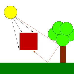
In the real world, the light that reaches an object is a combination of both direct and indirect light. Direct light is that which comes straight from a light source, while indirect light is the result of light rays hitting other surfaces in the scene, bouncing off of them and eventually reaching the object as a result, maybe after multiple reflections from other objects. Because each time a ray of light hits a surface it loses part of its energy, indirect light reflection is less bright than direct light reflection and its color might have been altered. The contrast between surfaces that are directly hit by the light source and surfaces that only receive indirect light is what creates shadows. A shadow isn’t but the part of a scene that doesn’t receive direct light but might still receive some amount of (less intense) indirect light.

Light in the digital world

Unfortunately, implementing realistic light behavior like that is too expensive, specially for real-time applications, so instead we use simplifications that can produce similar results with much lower computing requirements. The Phong reflection model in particular describes the light reflected from surfaces or emitted by light sources as the combination of 3 components: diffuse, ambient and specular. The model also requires information about the direction in which a particular surface is facing, provided via vectors called surface normals. Let’s introduce each of these concepts:

Surface normals

When we study the behavior of light, we notice that the direction in which surfaces reflect incoming light affects our perception of the surface. For example, if we lit a shiny surface (such as a piece of metal) using a strong light shource so that incoming light is reflected off the surface in the exact opposite direction in which we are looking at it, we will see a strong reflection in the form of highlights. If we move around so that we look at the same surface from a different angle, then we will see the reflection get dimmer and the highlights will eventually disappear. In order to model this behavior we need to know the direction in which the surfaces we render reflect incoming light. The way to do this is by associating vectors called normals with the surfaces we render so that shaders can use that information to produce lighting calculations akin to what we see in the natural world.

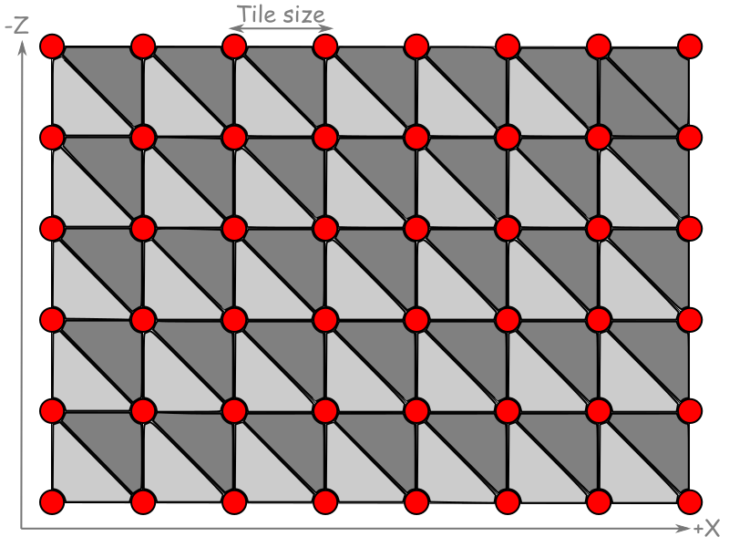
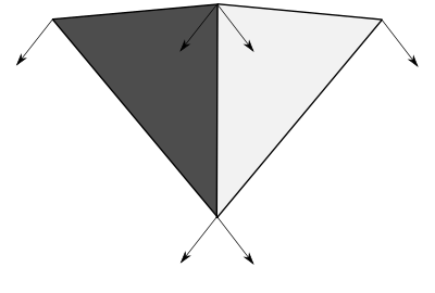
Usually, modeling programs can compute normal vectors for us, even model loading libraries can do this work automatically, but some times, for example when we define vertex meshes programatically, we need to define them manually. I won’t covere here how to do this in the general, you can see this article from Khronos if you’re interested in specific algorithms, but I’ll point out something relevant: given a plane, we can compute normal vectors in two opposite directions, one is correct for the front face of the plane/polygon and the other one is correct for the back face, so make sure that if you compute normals manually, you use the correct direction for each face, otherwise you won’t be reflecting light in the correct direction and results won’t be as you expect.

In most scenarios, we only render the front faces of the polygons (by enabling back face culling) and thus, we only care about one of the normal vectors (the one for the front face).

Another thing to notice about normal vectors is that they need to be transformed with the model to be correct for transformed models: if we rotate a model we need to rotate the normals too, since the faces they represent are now rotated and thus, their normal directions have rotated too. Scaling also affects normals, specifically if we don’t use regular scaling, since in that case the orientation of the surfaces may change and affect the direction of the normal vector. Because normal vectors represent directions, their position in world space is irrelevant, so for the purpose of lighting calculations, a normal vector such as (1, 0, 0) defined for a surface placed at (0, 0, 0) is still valid to represent the same surface at any other position in the world; in other words, we do not need to apply translation transforms to our normal vectors.

In practice, the above means that we want to apply the rotation and scale transforms from our models to their normal vectors, but we can skip the translation transform. The matrix representing these transforms is usually called the normal matrix. We can compute the normal matrix from our model matrix by computing the transpose of the inverse of the 3×3 submatrix of the model matrix. Usually, we’d want to compute this matrix in the application and feed it to our vertex shader like we do with our model matrix, but for reference, here is how this can be achieved in the shader code itself, plus how to use this matrix to transform the original normal vectors:

mat3 NormalMatrix = transpose(inverse(mat3(ModelMatrix)));
vec3 out_normal = normalize(NormalMatrix * in_normal);

Notice that the code above normalizes the resulting normal before it is fed to the fragment shader. This is important because the rasterizer will compute normals for all fragments in the surface automatically, and for that it will interpolate between the normals for each vertex we emit. For the interpolated normals to be correct, all vertex normals we output in the vertex shader must have the same length, otherwise the larger normals will deviate the direction of the interpolated vectors towards them because their larger size will increase their weight in the interpolation computations.

Finally, even if we emit normalized vectors in the vertex shader stage, we should note that the interpolated vectors that arrive to the fragment shader are not guaranteed to be normalized. Think for example of the normal vectors (1, 0, 0) and (0, 1, 0) being assigned to the two vertices in a line primitive. At the half-way point in between these two vertices, the interpolator will compute a normal vector of (0.5, 0.5, 0), which is not unit-sized. This means that in the general case, input normals in the fragment shader will need to be normalized again even if have normalized vertex normals at the vertex shader stage.

Diffuse reflection

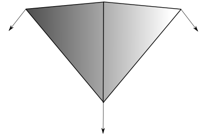
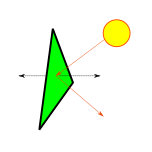
The diffuse component represents the reflection produced from direct light. It is important to notice that the intensity of the diffuse reflection is affected by the angle between the light coming from the source and the normal of the surface that receives the light. This makes a surface looking straight at the light source be the brightest, with reflection intensity dropping as the angle increases:

In order to compute the diffuse component for a fragment we need its normal vector (the direction in which the surface is facing), the vector from the fragment’s position to the light source, the diffuse component of the light and the diffuse reflection of the fragment’s material:

vec3 normal = normalize(surface_normal);
vec3 pos_to_light_norm = normalize(pos_to_light);
float dp_reflection = max(0.0, dot(normal, pos_to_light_norm));
vec3 diffuse = material.diffuse * light.diffuse * dp_reflection;

Basically, we multiply the diffuse component of the incoming light with the diffuse reflection of the fragment’s material to produce the diffuse component of the light reflected by the fragment. The diffuse component of the surface tells how the object absorbs and reflects incoming light. For example, a pure yellow object (diffuse material vec3(1,1,0)) would absorb the blue component and reflect 100% of the red and green components of the incoming light. If the light is a pure white light (diffuse vec3(1,1,1)), then the observer would see a yellow object. However, if we are using a red light instead (diffuse vec3(1,0,0)), then the light reflected from the surface of the object would only contain the red component (since the light isn’t emitting a green component at all) and we would see it red.

As we said before though, the intensity of the reflection depends on the angle between the incoming light and the direction of the reflection. We account for this with the dot product between the normal at the fragment (surface_normal) and the direction of the light (or rather, the vector pointing from the fragment to the light source). Notice that because the vectors that we use to compute the dot product are normalized, dp_reflection is exactly the cosine of the angle between these two vectors. At an angle of 0º the surface is facing straight at the light source, and the intensity of the diffuse reflection is at its peak, since cosine(0º)=1. At an angle of 90º (or larger) the cosine will be 0 or smaller and will be clamped to 0, meaning that no light is effectively being reflected by the surface (the computed diffuse component will be 0).

Ambient reflection

Computing all possible reflections and bounces of all rays of light from each light source in a scene is way too expensive. Instead, the Phong model approximates this by making indirect reflection from a light source constant across the scene. In other words: it assumes that the amount of indirect light received by any surface in the scene is the same. This eliminates all the complexity while still producing reasonable results in most scenarios. We call this constant factor ambient light.

Adding ambient light to the fragment is then as simple as multiplying the light source’s ambient light by the material’s ambient reflection. The meaning of this product is exactly the same as in the case of the diffuse light, only that it affects the indirect light received by the fragment:

vec3 ambient = material.ambient * light.ambient;

Specular reflection

Very sharp, smooth surfaces such as metal are known to produce specular highlights, which are those bright spots that we can see on shiny objects. Specular reflection depends on the angle between the observer’s view direction and the direction in which the light is reflected off the surface. Specifically, the specular reflection is strongest when the observer is facing exactly in the opposite direction in which the light is reflected. Depending on the properties of the surface, the specular reflection can be more or less focused, affecting how the specular component scatters after being reflected. This property of the material is usually referred to as its shininess.

Implementing specular reflection requires a bit more of work:

vec3 specular = vec3(0);
vec3 light_dir_norm = normalize(vec3(light.direction));
if (dot(normal, -light_dir_norm) >= 0.0) {
   vec3 reflection_dir = reflect(light_dir_norm, normal);
   float shine_factor = dot(reflection_dir, normalize(in_view_dir));
   specular = light.specular.xyz * material.specular.xyz *
         pow(max(0.0, shine_factor), material.shininess.x);
}

Basically, the code above checks if there is any specular reflection at all by computing the cosine of the angle between the fragment’s normal and the direction of the light (notice that, once again, both vectors are normalized prio to using them in the call to dot()). If there is specular reflection, then we compute how shiny the reflection is perceived by the viewer based on the angle between the vector from this fragment to the observer (in_view_dir) and the direction of the light reflected off the fragment’s surface (reflection_dir). The smaller the angle, the more parallel the directions are, meaning that the camera is receiving more reflection and the specular component received is stronger. Finally, we modulate the result based on the shininess of the fragment. We can compute in_view_dir in the vertex shader using the inverse of the View matrix like this:

mat4 ViewInv = inverse(View);
out_view_dir =
   normalize(vec3(ViewInv * vec4(0.0, 0.0, 0.0, 1.0) - world_pos));

The code above takes advantage of the fact that camera transformations are an illusion created by applying the transforms to everything else we render. For example, if we want to create the illusion that the camera is moving to the right, we just apply a translation to everything we render so they show up a bit to the left. This is what our View matrix achieves. From the point of view of GL or Vulkan, the camera is always fixed at (0,0,0). Taking advantage of this, we can compute the position of the virtual observer (the camera) in world space coordinates by applying the inverse of our camera transform to its fixed location (0,0,0). This is what the code above does, where world_pos is the position of this vertex in world space and View is the camera’s view matrix.

In order to produce the final look of the scene according to the Phong reflection model, we need to compute these 3 components for each fragment and add them together:

out_color  = vec4(diffuse + ambient + specular, 1.0)

Attenuation

In most scenarios, light intensity isn’t constant across the scene. Instead, it is brightest at its source and gets dimmer with distance. We can easily model this by adding an attenuation factor that is multiplied by the distance from the fragment to the light source. Typically, the intensity of the light decreases quite fast with distance, so a linear attenuation factor alone may not produce the best results and a quadratic function is preferred:

float attenuation = 1.0 /
    (light.attenuation.constant +
     light.attenuation.linear * dist +
     light.attenuation.quadratic * dist * dist);

diffuse = diffuse * attenuation;
ambient = ambient * attenuation;
specular = specular * attenuation;

Of course, we may decide not to apply attenuation to the ambient component at all if we really want to make it look like it is constant across the scene, however, do notice that when multiple light sources are present, the ambient factors from each source will accumulate and may produce too much ambient light unless they are attenuated.

Types of lights

When we model a light source we also need to consider the kind of light we are manipulating:

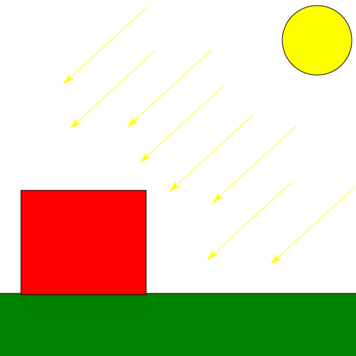
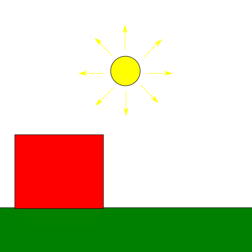
Directional lights

These are light sources that emit rays that travel along a specific direction so that all are parallel to each other. We typically use this model to represent bright, distant light sources that produce constant light across the scene. An example would be the sun light. Because the distance to the light source is so large compared to distances in the scene, the attenuation factor is irrelevant and can be discarded. Another particularity of directional light sources is that because the light rays are parallel, shadows casted from them are regular (we will talk more about this once we cover shadow mapping in future posts).

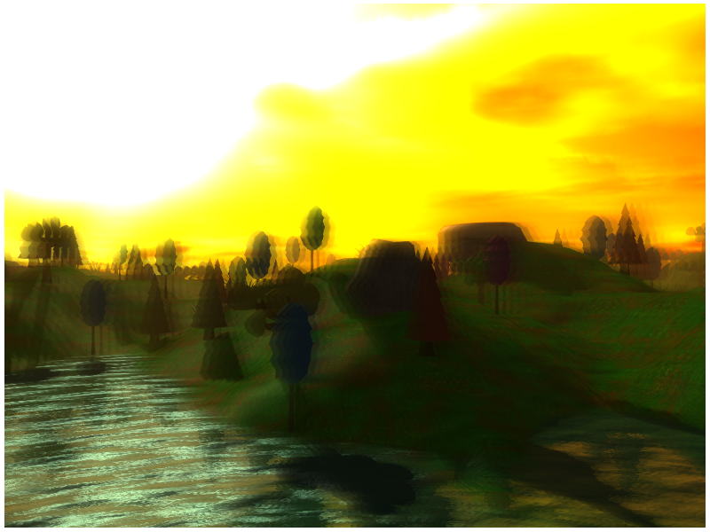
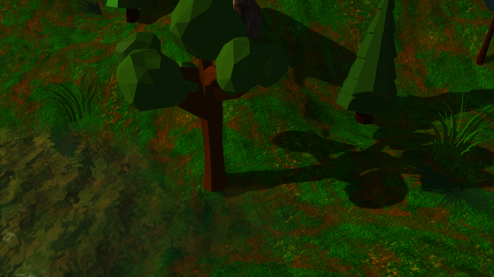
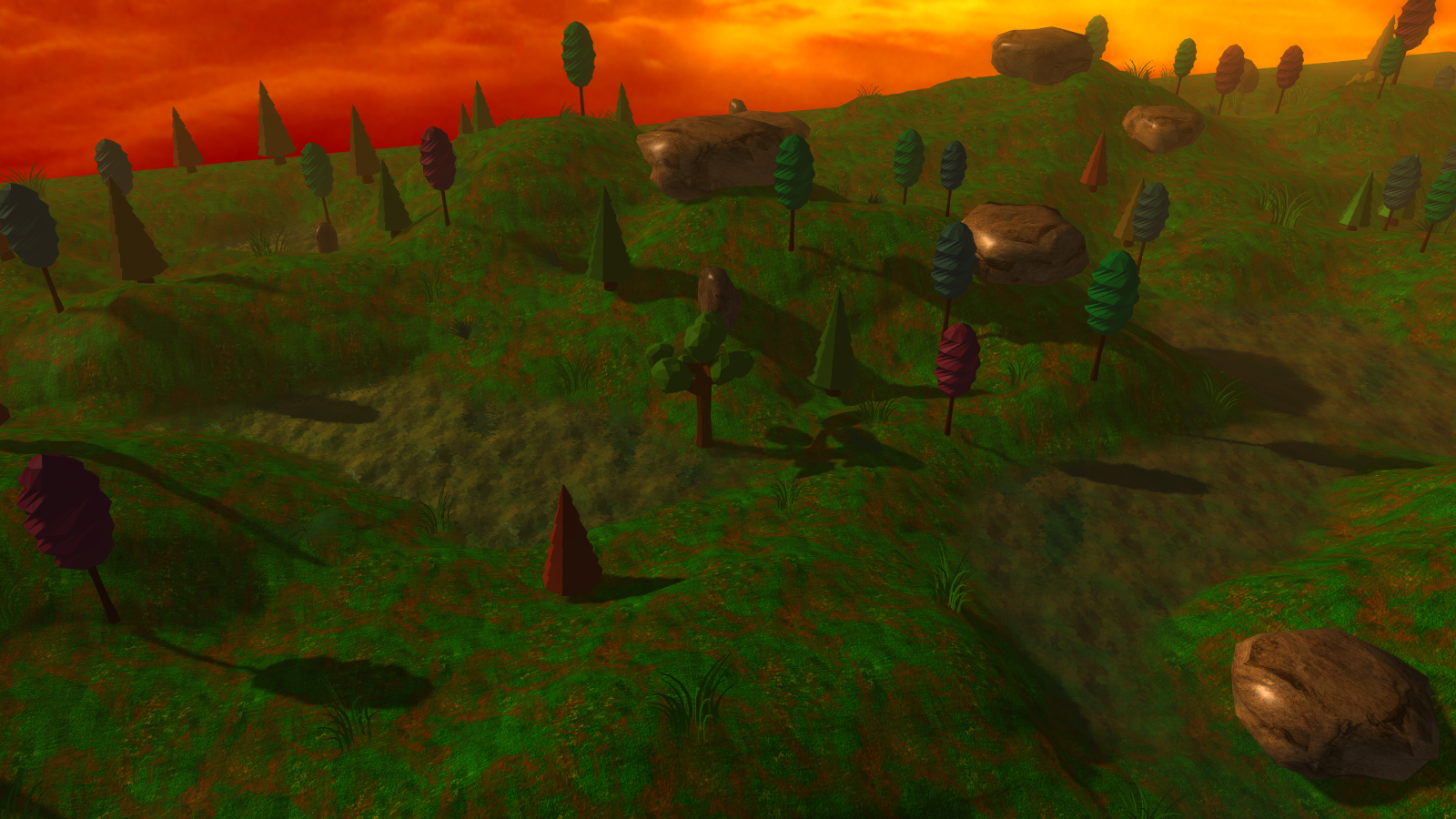
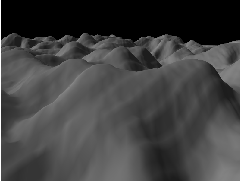
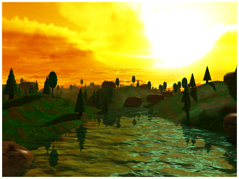
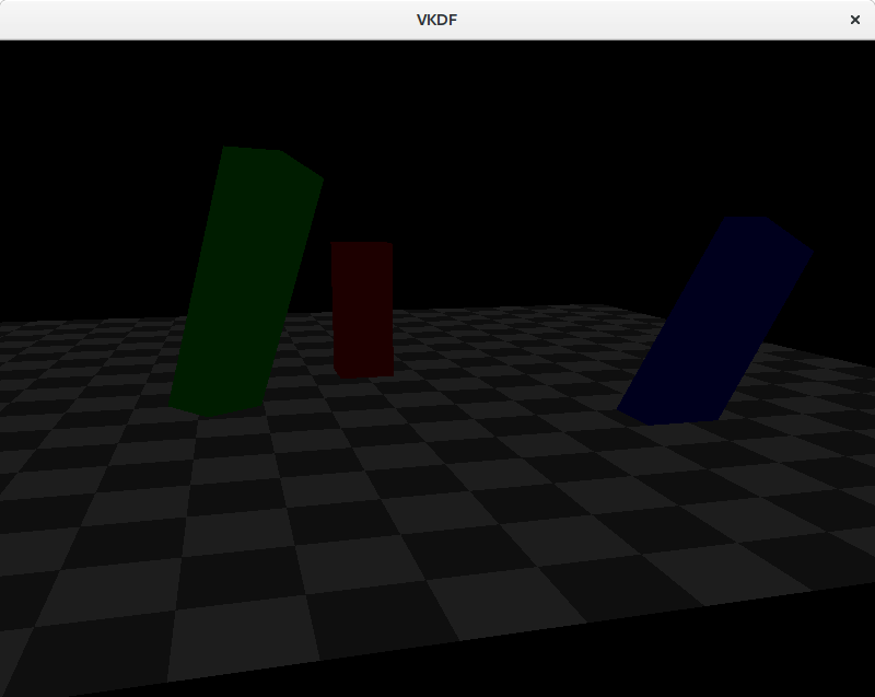
If we had used a directional light in the scene, it would look like this:

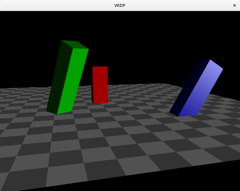
Notice how the brightness of the scene doesn’t lower with the distance to the light source.

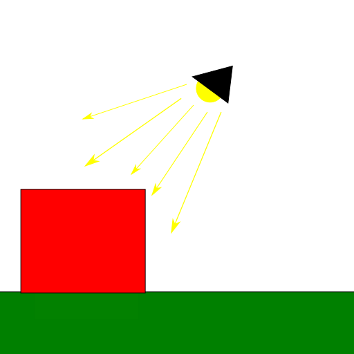
Point lights

These are light sources for which light originates at a specific position and spreads outwards in all directions. Shadows casted by point lights are not regular, instead they are projected. An example would be the light produced by a light bulb. The attenuation code I showed above would be appropriate to represent point lights.

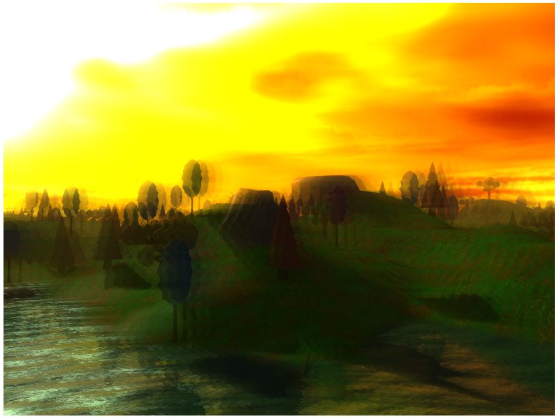
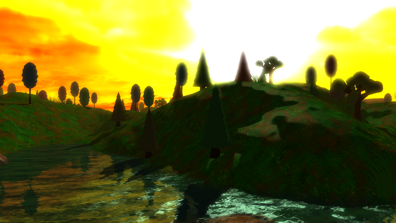
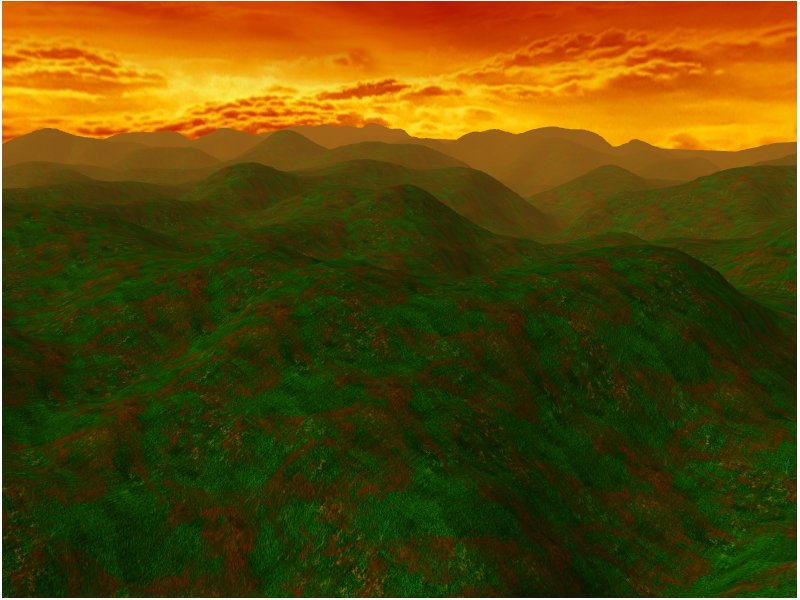
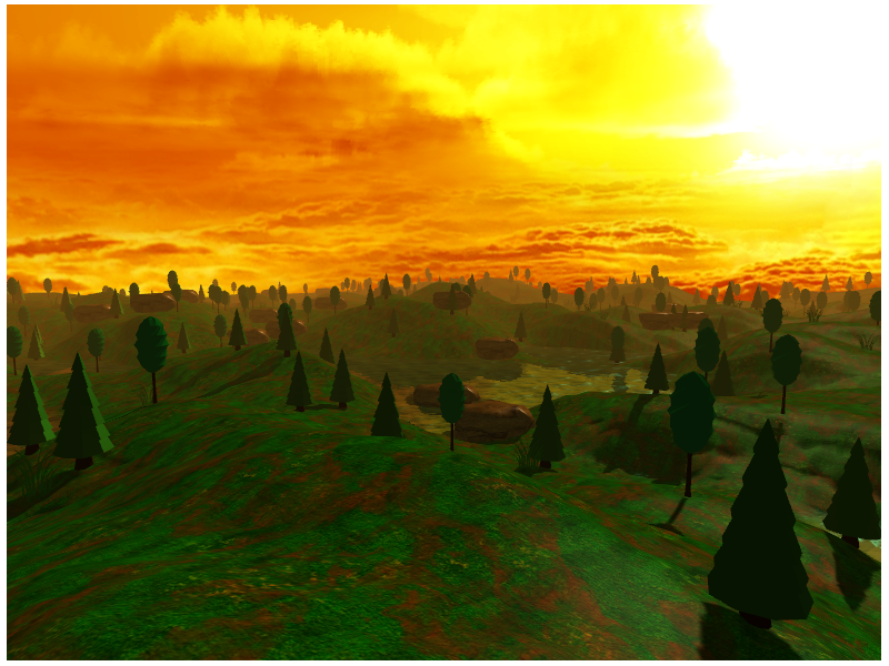
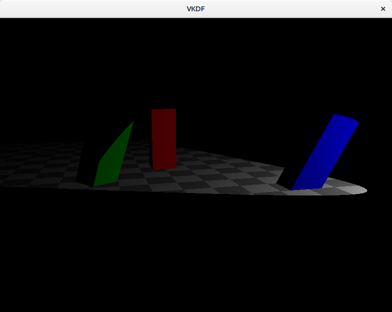
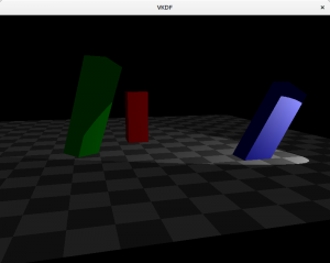
Here is how the scene would look like with a point light:

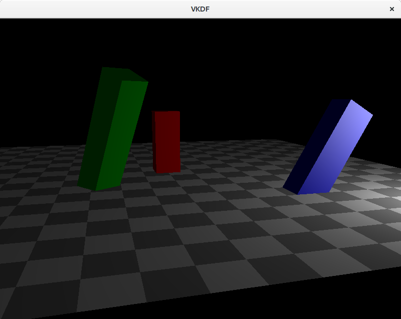
In this case, we can see how attenuation plays a factor and brightness lowers as we walk away from the light source (which is close to the blue cuboid).

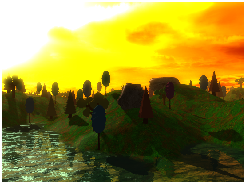
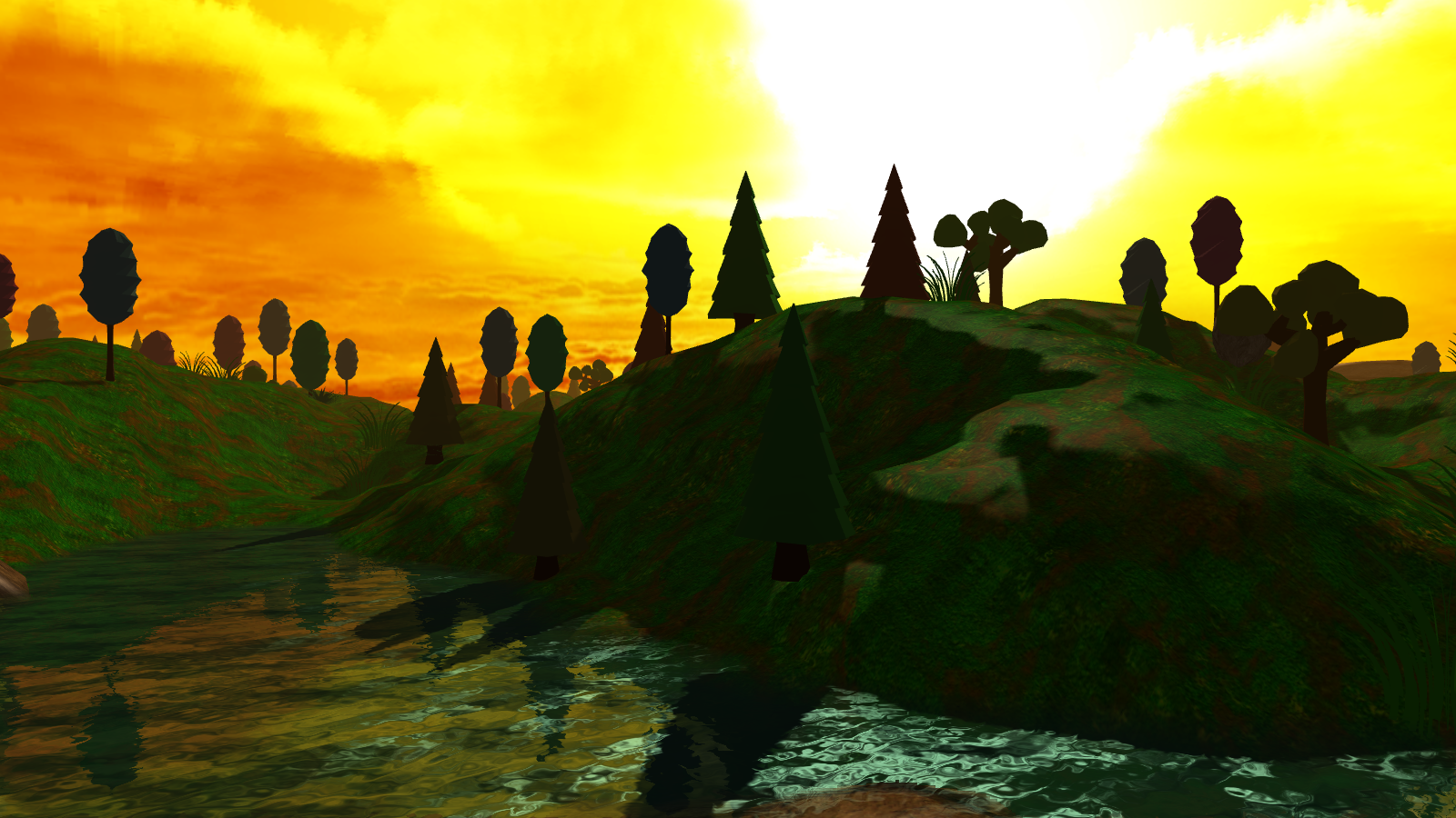
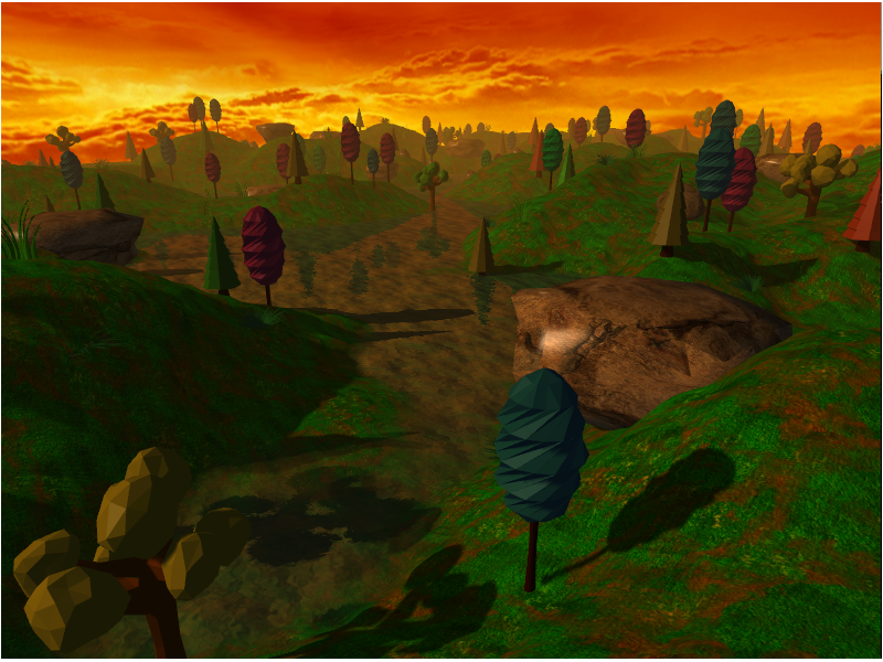
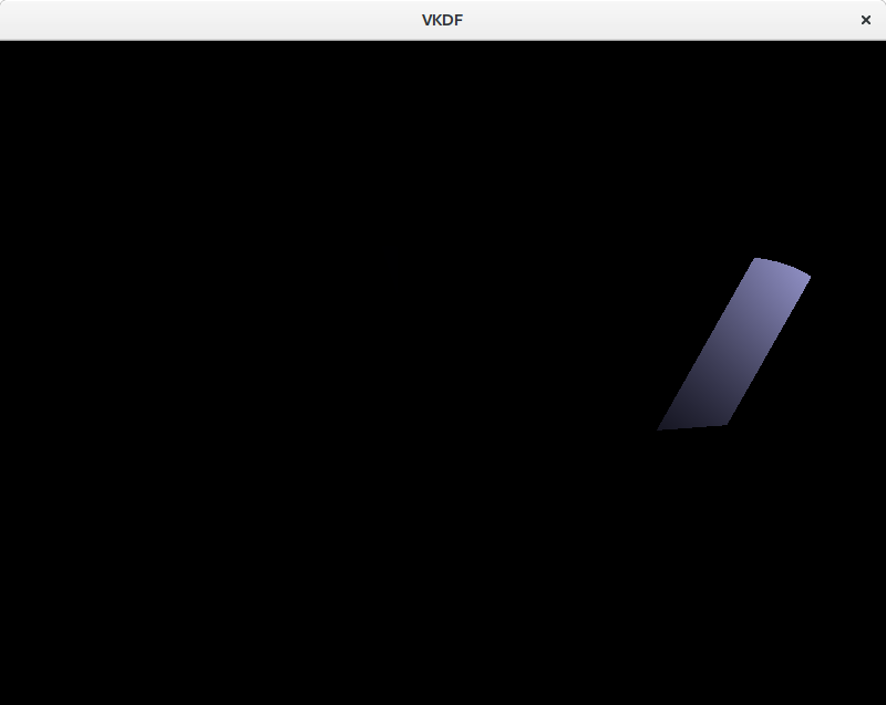
Spotlights

This is the light source I used to illustrate the diffuse, ambient and specular components. They are similar to point lights, is the sense that light originates from a specific point in space and spreads outwards, however, instead of scattering in all directions, rays scatter forming a cone with the tip at the origin of the light. The angle formed by the lights’s direction and the sides of the cone is usually called the cutoff angle, because not light is casted outside its limits. Flashlights are a good example of this type of light.

In order to create spotlights we need to consider the cutoff angle of the light and make sure that no diffuse or specular component is reflected by a fragment which is beyond the cutoff threshold:

vec3 light_to_pos_norm = -pos_to_light_norm;
float dp = dot(light_to_pos_norm, light_dir_norm);
if (dp <= light.cutoff) {
   diffuse = vec3(0);
   specular = vec3(0);
}

In the code above we compute the cosine of the angle between the light’s direction and the vector from the light to the fragment (dp). Here, light.cutoff represents the cosine of the spotlight’s cutoff angle too, so when dp is smaller it means that the fragment is outside the light cone emitted by the spotlight and we remove its diffuse and specular reflections completely.

Multiple lights

Handling multiple lights is easy enough: we only need to compute the color contribution for each light separately and then add all of them together for each fragment (pseudocode):

vec3 fragColor = vec3(0);
foreach light in lights
    fragColor += compute_color_for_light(light, ...);
...

Of course, light attenuation plays a vital role here to limit the area of influence of each light so that scenes where we have multiple lights don’t get too bright.

An important thing to notice above the pseudocode above is that this process involves looping through costy per-fragment light computations for each light source, which can lead to important performance hits as the number of lights in the scene increases. This shading model, as described here, is called forward rendering and it has the benefit that it is very simple to implement but its downside is that we may incur in many costy lighting computations for fragments that, eventually, won’t be visible in the screen (due to them being occluded by other fragments). This is particularly important when the number of lights in the scene is quite large and its complexity makes it so that there are many occluded fragments. Another technique that may be more suitable for these situations is called deferred rendering, which postpones costy shader computations to a later stage (hence the word deferred) in which we only evaluate them for fragments that are known to be visible, but that is a topic for another day, in this series we will focus on forward rendering only.

Lights and shadows

For the purpose of shadow mapping in particular we should note that objects that are directly lit by the light source reflect all 3 of the light components, while objects in the shadow only reflect the ambient component. Because objects that only reflect ambient light are less bright, they appear shadowed, in similar fashion as they would in the real world. We will see the details how this is done in the next post, but for the time being, keep this in mind.

Source code

The scene images in this post were obtained from a simple shadow mapping demo I wrote in Vulkan. The source code for that is available here, and it includes also the shadow mapping implementation that I’ll cover in the next post. Specifically relevant to this post are the scene vertex and fragment shaders where lighting calculations take place.

Conclusions

In order to represent shadows we first need a means to represent light. In this post we discussed the Phong reflection model as a simple, yet effective way to model light reflection in a scene as the addition of three separate components: diffuse, ambient and specular. Once we have a representation of light we can start discussing shadows, which are parts of the scene that only receive ambient light because other objects occlude the diffuse and specular components of the light source.

2017 starts with good news for Intel Haswell users: it has been a long time coming, but we have finally landed GL_ARB_gpu_shader_fp64 for this platform. Thanks to Matt Turner for reviewing the huge patch series!

Maybe you are not particularly excited about GL_ARB_gpu_shader_fp64, but that does not mean this is not an exciting milestone for you if you have a Haswell GPU (or even IvyBridge, read below): this extension was the last piece missing to finally bring Haswell to expose OpenGL 4.0!

If you want to give it a try but you don’t want to build the driver from the latest Mesa sources, don’t worry: the feature freeze for the Mesa 13.1 release is planned to happen in just a few days and the current plan is to have the release in early February, so if things go according to plan you won’t have to wait too long for an official release.

But that is not all, now that we have landed Fp64 we can also send for review the implementation of GL_ARB_vertex_attrib_64bit. This could be a very exciting milestone, since I believe this is the only thing missing for Haswell to have all the extensions required for OpenGL 4.5!

You might be wondering about IvyBridge too, and 2017 also starts with good news for IvyBridge users. Landing Fp64 for Haswell allowed us to send for review the IvyBridge patches we had queued up for GL_ARB_gpu_shader_fp64 which will bring IvyBridge up to OpenGL 4.0. But again, that is not all, once we land Fp64 we should also be able to send the patches for GL_vertex_attrib_64bit and get IvyBridge up to OpenGL 4.2, so look forward to this in the near future!

We have been working hard on Fp64 and Va64 during a good part of 2016, first for Broadwell and later platforms and later for Haswell and IvyBridge; it has been a lot of work so it is exciting to see all this getting to the last stages and on its way to the hands of the final users.

All this has only been possible thanks to Intel’s sponsoring and the great support and insight that our friends there have provided throughout the development and review processes, so big thanks to all of them and also to the team at Igalia that has been involved in the development with me.

As usual, it can be turned on and off at build-time and there is some configuration available as well to control how the effect works. Here are some screen-shots:

Motion blur is a technique used to make movement feel smoother than it actually is and is targeted at hiding the fact that things don’t move in continuous fashion, but rather, at fixed intervals dictated by the frame rate. For example, a fast moving object in a scene can “leap” many pixels between consecutive frames even if we intend for it to have a smooth animation at a fixed speed. Quick camera movement produces the same effect on pretty much every object on the scene. Our eyes can notice these gaps in the animation, which is not great. Motion blur applies a slight blur to objects across the direction in which they move, which aims at filling the animation gaps produced by our discrete frames, tricking the brain into perceiving a smoother animation as result.

In my demo there are no moving objects other than the sky box or the shadows, which are relatively slow objects anyway, however, camera movement can make objects change screen-space positions quite fast (specially when we rotate the view point) and the motion- blur effect helps us perceive a smoother animation in this case.

I will try to cover the actual implementation in some other post but for now I’ll keep it short and leave it to the images above to showcase what the filter actually does at different configuration settings. Notice that the smoothing effect is something that can only be perceived during motion, so still images are not the best way to showcase the result of the filter from the perspective of the viewer, however, still images are a good way to freeze the animation and see exactly how the filter modifies the original image to achieve the smoothing effect.

Bloom Filter

The bloom filter makes bright objects glow and bleed through other objects positioned in between them and the camera. It is a common post-processing effect used all the time in video games and animated movies. The demo supports a couple of configuration options that control the intensity and behavior of the filter, here are some screenshots with different settings:

I particularly like the glow effect that this brings to the specular reflections on the water surface, although to really appreciate that you need to run the demo and see it in motion.

Cascaded Shadow Maps

I should really write a post about basic shadow mapping before going into the details of Cascaded Shadow Maps, so for now I’ll just focus on the problem they try to solve.

One of the problems with shadow mapping is rendering high resolution shadows, specially for shadows that are rendered close to the camera. Generally, basic shadow mapping provides two ways in which we can improve the resolution of the shadows we render:

1. Increase the resolution of the shadow map textures. This one is obvious but comes at a high performance (and memory) hit.

2. Reduce the distance at which we can render shadows. But this is not ideal of course.

One compromise solution is to notice that, as usual with 3D computer graphics, it is far more important to render nearby objects in high quality than distant ones.

Cascaded Shadow Maps allow us to use different levels of detail for shadows that are rendered at different distances from the camera. Instead of having a single shadow map for all the shadows, we split the viewing frustum into slices and render shadows in each slice to a different shadow map.

There are two immediate benefits of this technique:

1. We have flexibility to define the resolution of the shadow maps for each level of the cascade, allowing us, for example, to increase the resolution of the levels closest to the camera and maybe reduce those that are further away.

2. Each level only records shadows in a slice of the viewing frustum, which increases shadow resolution even if we keep the same texture resolution we used with the original shadow map implementation for each shadow map level.

This approach also has some issues:

1. We need to render multiple shadow maps, which can be a serious performance hit depending on the resolutions of the shadow maps involved. This is why we usually lower the resolution of the shadow maps as distance from the camera increases.

2. As we move closer to or further from shadowed objects we can see the changes in shadow quality pop-in. Of course we can control this by avoiding drastic quality changes between consecutive levels in the cascade.

Here is an example that illustrates the second issue (in this case I have lowered the resolution of the 2nd and 3d cascade levels to 50% and 25% respectively so the effect was more obvious). The screenshots show the rendering of the shadows at different distances. We can see how the shadows in the close-up shot are very sharp and as the distance increases they become blurrier due to the use of a lower resolution shadow map:

The demo supports up to 4 shadow map levels although the default configuration is to use 3. The resolution of each level can be configured separately too, in the default configuration I lowered the shadow resolution of the second and third levels to 75% and 50% respectively. If we configure the demo to run on a single level (with 100% texture resolution), we are back to the original shadow map implementation, so it is easy to experiment with both techniques.

I intend to cover the details behind shadow mapping and the implementation of the bloom filter in more detail in a future post, so again, stay tuned for more!

In this post I’ll discuss how I setup and render terrain mesh in the OpenGL terrain rendering demo. Most of the relevant code for this is in the ter-terrain.cpp file.

Setting up a grid of vertices

Unless you know how to use a 3D modeling program properly, a reasonable way to create a decent mesh for a terrain consists in using a grid of vertices and elevate them according to a height map image. In order to create the grid we only need to decide how many rows and columns we want. This, in the end, determines the number of polygons and the resolution of the terrain.

We need to map these vertices to world coordinates too. We do that by defining a tile size, which is the distance between consecutive vertices in world units. Larger tile sizes increase the size of the terrain but lower the resolution by creating larger polygons.

The image below shows an 8×6 grid that defines 35 tiles. Each tile is rendered using 2 triangles:

The next step is to elevate these vertices so we don’t end up with a boring flat surface. We do this by sampling the height map image for each vertex in the grid. A height map is a gray scale image where the values of the pixels represent altitudes at different positions. The closer the color is to white, the more elevated it is.

Adding more vertices to the grid increases the number of sampling points from the height map and reduces the sampling distances, leading to a smoother and more precise representation of the height map in the resulting terrain.

Of course, we still need to map the height map samples (gray scale colors) to altitudes in world units. In the demo I do this by normalizing the color values to [-1,+1] and then applying a scale factor to compute the altitude values in world space. By playing with the scaling factor we can make our terrain look more or less abrupt.

For reference, the height map sampling is implemented in ter_terrain_set_heights_from_texture().

Creating the mesh

At this point we know the full position (x, y, z) in world coordinates of all the vertices in our grid. The next step is to build the actual triangle mesh that we will use to render the terrain and the normal vectors for each triangle. This process is described below and is implemented in the ter_terrain_build_mesh() function.

Computing normals

In order to get nice lighting on our terrain we need to compute normals for each vertex in the mesh. A simple way to achieve this is would be to compute the normal for each face (triangle) and use that normal for each vertex in the triangle. This works, but it has 3 problems:

1. Every vertex of each triangle has the same exact normal, which leads to a rather flat result.

2. Adjacent triangles with different orientations showcase abrupt changes in the normal value, leading to significantly different lighting across the surfaces that highlight the individual triangles in the mesh.

3. Because each vertex in the mesh can have a different normal value for each triangle it participates in, we need to replicate the vertices when we render, which is not optimal.

Alternatively, we can compute the normals for each vertex considering the heights of its neighboring vertices. This solves all the problems mentioned above and leads to much better results thanks to the interpolation of the normal vectors across the triangles, which leads to smooth lighting reflection transitions:

The implementation for this is in the function calculate_normal(), which takes the column and row indices of the vertex in the grid and calculates the Y coordinate by sampling the heights of the 4 nearby vertices in the grid.

Preparing the draw call

Now that we know the positions of all the vertices and their normal vectors we have all the information that we need to render the terrain. We still have to decide how exactly we want to render all the polygons.

The simplest way to render the terrain using a single draw call is to setup a vertex buffer with data for each triangle in the mesh (including position and normal information) and use GL_TRIANGLES for the primitive of the draw call. This, however, is not the best option from the point of view of performance.

Because the terrain will typically contain a large number of vertices and most of them participate in multiple triangles, we end up uploading a large amount of vertex data to the GPU and processing a lot of vertices in the draw call. The result is large memory requirements and suboptimal performance.

For reference, the terrain I used in the demo from my original post used a 251×251 grid. This grid represents 250×250 tiles, each one rendered as two triangles (6 vertices/tile), so we end up with 250x250x6=375,000 vertices. For each of these vertices we need to upload 24 bytes of vertex data with the position and normal, so we end up with a GPU buffer that is almost 9MB large.

One obvious way to reduce this is to render the terrain using triangle strips. The problem with this is that in theory, we can’t render the terrain with just one strip, we would need one strip (and so, one draw call) per tile column or one strip per tile row. Fortunately, we can use degenerate triangles to link separate strips for each column into a single draw call. With this we trim down the number of vertices to 126,000 and the size of the buffer to a bit below 3 MB. This alone produced a 15%-20% performance increase in the demo.

We can do better though. A lot of the vertices in the terrain mesh participate in various triangles across the large triangle strip in the draw call, so we can reduce memory requirements by using an index buffer to render the strip. If we do this, we trim things down to 63,000 vertices and ~1.5MB. This added another 4%-5% performance bonus over the original implementation.

Clipping

So far we have been rendering the full mesh of the terrain in each frame and we do this by uploading the vertex data to the GPU just once (for example in the first frame). However, depending on where the camera is located and where it is looking at, just a fraction of the terrain may be visible.

Although the GPU will discard all the geometry and fragments that fall outside the viewport, it still has to process each vertex in the vertex shader stage before it can clip non-visible triangles. Because the number of triangles in the terrain is large, this is suboptimal and to address this we want to do CPU-side clipping before we render.

Doing CPU-side clippig comes with some additional complexities though: it requires that we compute the visible region of the terrain and upload new vertex data to the GPU in each frame preventin GPU stalls.

In the demo, we implement the clipping by computing a quad sub-region of the terrain that includes the visible area that we need to render. Once we know the sub-region that we want to render, we compute the new indices of the vertices that participate in the region so we can render it using a single triangle strip. Finally, we upload the new index data to the index buffer for use in the follow-up draw call.

Avoiding GPU stalls

Although all the above is correct, it actually leads, as described, to much worse performance in general. The reason for this is that our uploads of vertex data in each frame lead to frequent GPU stalls. This happens in two scenarios:

1. In the same frame, because we need to upload different vertex data for the rendering of the terrain for the shadow map and the scene (the shadow map renders the terrain from the point of view of the light, so the visible region of the terrain is different). This creates stalls because the rendering of the terrain for the shadow map might not have completed before we attempt to upload new data to the index buffer in order to render the terrain for the scene.

2. Between different frames. Because the GPU might not be completely done rendering the previous frame (and thus, stills needs the index buffer data available) before we start preparing the next frame and attempt to upload new terrain index data for it.

In the case of the Intel Mesa driver, these GPU stalls can be easily identified by using the environment variable INTEL_DEBUG=perf. When using this, the driver will detect these situations and produce warnings informing about the stalls, the buffers affected and the regions of the buffers that generate the stall, such as:

Stalling on glBufferSubData(0, 503992) (492kb) to a busy (0-1007984)
buffer object.  Use glMapBufferRange() to avoid this.

The solution to this problem that I implemented (other than trying to put as much work as possible between read/write accesses to the index buffer) comes in two forms:

1. Circular buffers

In this case, we allocate a larger buffer than we need so that each subsequent upload of new index data happens in a separate sub-region of the allocated buffer. I set up the demo so that each circular buffer is large enough to hold the index data required for all updates of the index buffer happening in each frame (the shadow map and the scene).

2. Multi-buffering

We allocate more than one circular buffer. When we don’t have enough free space at the end of the current buffer to upload the new index buffer data, we upload it to a different circular buffer instead. When we run out of buffers we circle back to the first one (which at this point will hopefully be free to be re-used again).

So why not just use a single, very large circular buffer? Mostly because there are limits to the size of the buffers that the GPU may be able to handle correctly (or efficiently). Also, why not having many smaller independent buffers instead of circular buffers? That would work just fine, but using fewer, larger buffers reduces the number of objects we need to bind/unbind and is better to prevent memory fragmentation, so that’s a plus.

Final touches

We are almost done, at this point we only need to add a texture to the terrain surface, add some slight fog effect for distant pixels to create a more realistic look, add a skybox (it is important to choose the color of the fog so it matches the color of the sky!) and tweak the lighting parameters to get a nice result:

I hope to cover some of these aspects in future posts, so stay tuned for more!

I have been quite busy with various things in the last few weeks, but I have finally found some time to clean up and upload the code of the OpenGL terrain render demo to Github.

Since this was intended as a programming exercise I have not tried to be very elegant or correct during the implementation, so expect things like error handling to be a bit rough around the edges, but otherwise I think the code should be easy enough to follow.

Notice that I have only tested this on Intel GPUs. I know it works on NVIDIA too (thanks to Samuel and Chema for testing this) but there are a couple of rendering artifacts there, specifically at the edges of the skybox and some “pillars” showing up in the distance some times, probably because I am rendering one to many “rows” of the terrain and I end up rendering garbage. I may fix these some day.

The code I uploaded to the repository includes a few new features too:

• Model variants, which are basically color variations of the same model
• A couple of additional models (a new tree and plant) and a different rock type
• Collision detection, which makes navigating the terrain more pleasent

Here is a new screenshot:

In future posts I will talk a bit about some of the implementation details, so having the source code around will be useful. Enjoy!

Lately I have been working on a simple terrain OpenGL renderer demo, mostly to have a playground where I could try some techniques like shadow mapping and water rendering in a scenario with a non trivial amount of geometry, and I thought it would be interesting to write a bit about it.

But first, here is a video of the demo running on my old Intel IvyBridge GPU:

And some screenshots too:

Note that I did not create any of the textures or 3D models featured in the video.

With that out of the way, let’s dig into some of the technical aspects:

The terrain is built as a 251×251 grid of vertices elevated with a heightmap texture, so it contains 63,000 vertices and 125,000 triangles. It uses a single 512×512 texture to color the surface.

The water is rendered in 3 passes: refraction, reflection and the final rendering. Distortion is done via a dudv map and it also uses a normal map for lighting. From a geometry perspective it is also implemented as a grid of vertices with 750 triangles.

I wrote a simple OBJ file parser so I could load some basic 3D models for the trees, the rock and the plant models. The parser is limited, but sufficient to load vertex data and simple materials. This demo features 4 models with these specs:

• Tree A: 280 triangles, 2 materials.
• Tree B: 380 triangles, 2 materials.
• Rock: 192 triangles, 1 material (textured)
• Grass: 896 triangles (yes, really!), 1 material.

The scene renders 200 instances of Tree A another 200 instances of Tree B, 50 instances of Rock and 150 instances of Grass, so 600 objects in total.

Object locations in the terrain are randomized at start-up, but the demo prevents trees and grass to be under water (except for maybe their base section only) because it would very weird otherwise :), rocks can be fully submerged though.

Rendered objects fade in and out smoothly via alpha blending (so there is no pop-in/pop-out effect as they reach clipping planes). This cannot be observed in the video because it uses a static camera but the demo supports moving the camera around in real-time using the keyboard.

Lighting is implemented using the traditional Phong reflection model with a single directional light.

Shadows are implemented using a 4096×4096 shadow map and Percentage Closer Filter with a 3x3 kernel, which, I read is (or was?) a very common technique for shadow rendering, at least in the times of the PS3 and Xbox 360.

The demo features dynamic directional lighting (that is, the sun light changes position every frame), which is rather taxing. The demo also supports static lighting, which is significantly less demanding.

There is also a slight haze that builds up progressively with the distance from the camera. This can be seen slightly in the video, but it is more obvious in some of the screenshots above.

The demo in the video was also configured to use 4-sample multisampling.

As for the rendering pipeline, it mostly has 4 stages:

• Shadow map.
• Water refraction.
• Water reflection.
• Final scene rendering.

A few notes on performance as well: the implementation supports a number of configurable parameters that affect the framerate: resolution, shadow rendering quality, clipping distances, multi-sampling, some aspects of the water rendering, N-buffering of dynamic VBO data, etc.

The video I show above runs at locked 60fps at 800×600 but it uses relatively high quality shadows and dynamic lighting, which are very expensive. Lowering some of these settings (very specially turning off dynamic lighting, multisampling and shadow quality) yields framerates around 110fps-200fps. With these settings it can also do fullscreen 1600×900 with an unlocked framerate that varies in the range of 80fps-170fps.

That’s all in the IvyBridge GPU. I also tested this on an Intel Haswell GPU for significantly better results: 160fps-400fps with the “low” settings at 800×600 and roughly 80fps-200fps with the same settings used in the video.

So that’s it for today, I had a lot of fun coding this and I hope the post was interesting to some of you. If time permits I intend to write follow-up posts that go deeper into how I implemented the various elements of the demo and I’ll probably also write some more posts about the optimization process I followed. If you are interested in any of that, stay tuned for more.

In case you haven’t heard yet, with the recently announced Mesa 12.0 release, Intel gen8+ GPUs expose OpenGL 4.3, which is quite a big leap from the previous OpenGL 3.3!

Although this might surprise some, the truth is that even if the i965 driver only exposed OpenGL 3.3 it had been exposing many of the OpenGL 4.x extensions for quite some time, however, there was one OpenGL 4.0 extension in particular that was still missing and preventing the driver from exposing a higher version: ARB_gpu_shader_fp64 (fp64 for short). There was a good reason for this: it is a very large feature that has been in the works by Intel first and Igalia later for quite some time. We first started to work on this as far back as November 2015 and by that time Intel had already been working on it for months.

I won’t cover here what made this such a large effort because there would be a lot of stuff to cover and I don’t feel like spending weeks writing a series of posts on the subject :). Hopefully I will get a chance to talk about all that at XDC in September, so instead I’ll focus on explaining why we only have this working in gen8+ at the moment and the status of gen7 hardware.

The plan for ARB_gpu_shader_fp64 was always to focus on gen8+ hardware (Broadwell and later) first because it has better support for the feature. I must add that it also has fewer hardware bugs too, although we only found out about that later ;). So the plan was to do gen8+ and then extend the implementation to cover the quirks required by gen7 hardware (IvyBridge, Haswell, ValleyView).

At this point I should explain that Intel GPUs have two code generation backends: scalar and vector. The main difference between both backends is that the vector backend (also known as align16) operates on vectors (surprise, right?) and has native support for things like swizzles and writemasks, while the scalar backend (known as align1) operates on scalars, which means that, for example, a vec4 GLSL operation running is broken up into 4 separate instructions, each one operating on a single component. You might think that this makes the scalar backend slower, but that would not be accurate. In fact it is usually faster because it allows the GPU to exploit SIMD better than the vector backend.

The thing is that different hardware generations use one backend or the other for different shader stages. For example, gen8+ used to run Vertex, Fragment and Compute shaders through the scalar backend and Geometry and Tessellation shaders via the vector backend, whereas Haswell and IvyBridge use the vector backend also for Vertex shaders.

Because you can use 64-bit floating point in any shader stage, the original plan was to implement fp64 support on both backends. Implementing fp64 requires a lot of changes throughout the driver compiler backends, which makes the task anything but trivial, but the vector backend is particularly difficult to implement because the hardware only supports 32-bit swizzles. This restriction means that a hardware swizzle such as XYZW only selects components XY in a dvecN and therefore, there is no direct mechanism to access components ZW. As a consequence, dealing with anything bigger than a dvec2 requires more creative solutions, which then need to face some other hardware limitations and bugs, etc, which eventually makes the vector backend require a significantly larger development effort than the scalar backend.

Thankfully, gen8+ hardware supports scalar Geometry and Tessellation shaders and Intel‘s Kenneth Graunke had been working on enabling that for a while. When we realized that the vector fp64 backend was going to require much more effort than what we had initially thought, he gave a final push to the full scalar gen8+ implementation, which in turn allowed us to have a full fp64 implementation for this hardware and expose OpenGL 4.0, and soon after, OpenGL 4.3.

That does not mean that we don’t care about gen7 though. As I said above, the plan has always been to bring fp64 and OpenGL4 to gen7 as well. In fact, we have been hard at work on that since even before we started sending the gen8+ implementation for review and we have made some good progress.

Besides addressing the quirks of fp64 for IvyBridge and Haswell (yes, they have different implementation requirements) we also need to implement the full fp64 vector backend support from scratch, which as I said, is not a trivial undertaking. Because Haswell seems to require fewer changes we have started with that and I am happy to report that we have a working version already. In fact, we have already sent a small set of patches for review that implement Haswell‘s requirements for the scalar backend and as I write this I am cleaning-up an initial implementation of the vector backend in preparation for review (currently at about 100 patches, but I hope to trim it down a bit before we start the review process). IvyBridge and ValleView will come next.

The initial implementation for the vector backend has room for improvement since the focus was on getting it working first so we can expose OpenGL4 in gen7 as soon as possible. The good thing is that it is more or less clear how we can improve the implementation going forward (you can see an excellent post by Curro on that topic here).

You might also be wondering about OpenGL 4.1’s ARB_vertex_attrib_64bit, after all, that kind of goes hand in hand with ARB_gpu_shader_fp64 and we implemented the extension for gen8+ too. There is good news here too, as my colleague Juan Suárez has already implemented this for Haswell and I would expect it to mostly work on IvyBridge as is or with minor tweaks. With that we should be able to expose at least OpenGL 4.2 on all gen7 hardware once we are done.

So far, implementing ARB_gpu_shader_fp64 has been quite the ride and I have learned a lot of interesting stuff about how the i965 driver and Intel GPUs operate in the process. Hopefully, I’ll get to talk about all this in more detail at XDC later this year. If you are planning to attend and you are interested in discussing this or other Mesa stuff with me, please find me there, I’ll be looking forward to it.

Finally, I’d like to thank both Intel and Igalia for supporting my work on Mesa and i965 all this time, my igalian friends Samuel Iglesias, who has been hard at work with me on the fp64 implementation all this time, Juan Suárez and Andrés Gómez, who have done a lot of work to improve the fp64 test suite in Piglit and all the friends at Intel who have been helping us in the process, very especially Connor Abbot, Francisco Jerez, Jason Ekstrand and Kenneth Graunke.

In my previous post I introduced ARB_shader_storage_buffer, an OpenGL 4.3 feature that is coming soon to Mesa and the Intel i965 driver. While that post focused on explaining the features introduced by the extension, in this post I’ll dive into some of the implementation aspects, for those who are curious about this kind of stuff. Be warned that some parts of this post will be specific to Intel hardware.

Following the trail of UBOs

As I explained in my previous post, SSBOs are similar to UBOs, but they are read-write. Because there is a lot of code already in place in Mesa’s GLSL compiler to deal with UBOs, it made sense to try and reuse all the data structures and code we had for UBOs and specialize the behavior for SSBOs where that was needed, that allows us to build on code paths that are already working well and reuse most of the code.

That path, however, had some issues that bit me a bit further down the road. When it comes to representing these operations in the IR, my first idea was to follow the trail of UBO loads as well, which are represented as ir_expression nodes. There is a fundamental difference between the two though: UBO loads are constant operations because uniform buffers are read-only. This means that a UBO load operation with the same parameters will always return the same value. This has implications related to certain optimization passes that work based on the assumption that other ir_expression operations share this feature. SSBO loads are not like this: since the shader storage buffer is read-write, two identical SSBO load operations in the same shader may not return the same result if the underlying buffer storage has been altered in between by SSBO write operations within the same or other threads. This forced me to alter a number of optimization passes in Mesa to deal with this situation (mostly disabling them for the cases of SSBO loads and stores).

The situation was worse with SSBO stores. These just did not fit into ir_expression nodes: they did not return a value and had side-effects (memory writes) so we had to come up with a different way to represent them. My initial implementation created a new IR node for these, ir_ssbo_store. That worked well enough, but it left us with an implementation of loads and stores that was a bit inconsistent since both operations used very different IR constructs.

These issues were made clear during the review process, where it was suggested that we used GLSL IR intrinsics to represent load and store operations instead. This has the benefit that we can make the implementation more consistent, having both loads and stores represented with the same IR construct and follow a similar treatment in both the GLSL compiler and the i965 backend. It would also remove the need to disable or alter certain optimization passes to be SSBO friendly.

Read/Write coherence

One of the issues we detected early in development was that our reads and writes did not seem to work very well together: some times a read after a write would fail to see the last value written to a buffer variable. The problem here also spawned from following the implementation trail of the UBO path. In the Intel hardware, there are various interfaces to access memory, like the Sampling Engine and the Data Port. The former is a read-only interface and is used, for example, for texture and UBO reads. The Data Port allows for read-write access. Although both interfaces give access to the same memory region, there is something to consider here: if you mix reads through the Sampling Engine and writes through the Data Port you can run into cache coherence issues, this is because the caches in use by the Sampling Engine and the Data Port functions are different. Initially, we implemented SSBO load operations like UBO loads, so we used the Sampling Engine, and ended up running into this problem. The solution, of course, was to rewrite SSBO loads to go though the Data Port as well.

Parallel reads and writes

GPUs are highly parallel hardware and this has some implications for driver developers. Take a sentence like this in a fragment shader program:

float cx = 1.0;

This is a simple assignment of the value 1.0 to variable cx that is supposed to happen for each fragment produced. In Intel hardware running in SIMD16 mode, we process 16 fragments simultaneously in the same GPU thread, this means that this instruction is actually 16 elements wide. That is, we are doing 16 assignments of the value 1.0 simultaneously, each one is stored at a different offset into the GPU register used to hold the value of cx.

If cx was a buffer variable in a SSBO, it would also mean that the assignment above should translate to 16 memory writes to the same offset into the buffer. That may seem a bit absurd: why would we want to write 16 times if we are always assigning the same value? Well, because things can get more complex, like this:

float cx = gl_FragCoord.x;

Now we are no longer assigning the same value for all fragments, each of the 16 values assigned with this instruction could be different. If cx was a buffer variable inside a SSBO, then we could be potentially writing 16 different values to it. It is still a bit silly, since only one of the values (the one we write last), would prevail.

Okay, but what if we do something like this?:

int index = int(mod(gl_FragCoord.x, 8));
cx[index] = 1;

Now, depending on the value we are reading for each fragment, we are writing to a separate offset into the SSBO. We still have a single assignment in the GLSL program, but that translates to 16 different writes, and in this case the order may not be relevant, but we want all of them to happen to achieve correct behavior.

The bottom line is that when we implement SSBO load and store operations, we need to understand the parallel environment in which we are running and work with test scenarios that allow us to verify correct behavior in these situations. For example, if we only test scenarios with assignments that give the same value to all the fragments/vertices involved in the parallel instructions (i.e. assignments of values that do not depend on properties of the current fragment or vertex), we could easily overlook fundamental defects in the implementation.

Dealing with helper invocations

From Section 7.1 of the GLSL spec version 4.5:

“Fragment shader helper invocations execute the same shader code
as non-helper invocations, but will not have side effects that
modify the framebuffer or other shader-accessible memory.”

To understand what this means I have to introduce the concept of helper invocations: certain operations in the fragment shader need to evaluate derivatives (explicitly or implicitly) and for that to work well we need to make sure that we compute values for adjacent fragments that may not be inside the primitive that we are rendering. The fragment shader executions for these added fragments are called helper invocations, meaning that they are only needed to help in computations for other fragments that are part of the primitive we are rendering.

How does this affect SSBOs? Because helper invocations are not part of the primitive, they cannot have side-effects, after they had served their purpose it should be as if they had never been produced, so in the case of SSBOs we have to be careful not to do memory writes for helper fragments. Notice also, that in a SIMD16 execution, we can have both proper and helper fragments mixed in the group of 16 fragments we are handling in parallel.

Of course, the hardware knows if a fragment is part of a helper invocation or not and it tells us about this through a pixel mask register that is delivered with all executions of a fragment shader thread, this register has a bitmask stating which pixels are proper and which are helper. The Intel hardware also provides developers with various kinds of messages that we can use, via the Data Port interface, to write to memory, however, the tricky thing is that not all of them incorporate pixel mask information, so for use cases where you need to disable writes from helper fragments you need to be careful with the write message you use and select one that accepts this sort of information.

Vector alignments

Another interesting thing we had to deal with are address alignments. UBOs work with layout std140. In this setup, elements in the UBO definition are aligned to 16-byte boundaries (the size of a vec4). It turns out that GPUs can usually optimize reads and writes to multiples of 16 bytes, so this makes sense, however, as I explained in my previous post, SSBOs also introduce a packed layout mode known as std430.

Intel hardware provides a number of messages that we can use through the Data Port interface to write to memory. Each message has different characteristics that makes it more suitable for certain scenarios, like the pixel mask I discussed before. For example, some of these messages have the capacity to write data in chunks of 16-bytes (that is, they write vec4 elements, or OWORDS in the language of the technical docs). One could think that these messages are great when you work with vector data types, however, they also introduce the problem of dealing with partial writes: what happens when you only write to an element of a vector? or to a buffer variable that is smaller than the size of a vector? what if you write columns in a row_major matrix? etc

In these scenarios, using these messages introduces the need to mask the writes because you need to disable the channels in the vec4 element that you don’t want to write. Of course, the hardware provides means to do this, we only need to set the writemask of the destination register of the message instruction to select the right channels. Consider this example:

struct TB {
    float a, b, c, d;
};

layout(std140, binding=0) buffer Fragments {
   TB s[3];
   int index;
};

void main()
{
   s[0].d = -1.0;
}

In this case, we could use a 16-byte write message that takes 0 as offset (i.e writes at the beginning of the buffer, where s[0] is stored) and then set the writemask on that instruction to WRITEMASK_W so that only the fourth data element is actually written, this way we only write one data element of 4 bytes (-1) at offset 12 bytes (s[0].d). Easy, right? However, how do we know, in general, the writemask that we need to use? In std140 layout mode this is easy: since each element in the SSBO is aligned to a 16-byte boundary, we simply need to take the byte offset at which we are writing, divide it by 16 (to convert it to units of vec4) and the modulo of that operation is the byte offset into the chunk of 16-bytes that we are writing into, then we only have to divide that by 4 to get the component slot we need to write to (a number between 0 and 3).

However, there is a restriction: we can only set the writemask of a register at compile/link time, so what happens when we have something like this?:

s[i].d = -1.0;

The problem with this is that we cannot evaluate the value of i at compile/link time, which inevitably makes our solution invalid for this. In other words, if we cannot evaluate the actual value of the offset at which we are writing at compile/link time, we cannot use the writemask to select the channels we want to use when we don’t want to write a vec4 worth of data and we have to use a different type of message.

That said, in the case of std140 layout mode, since each data element in the SSBO is aligned to a 16-byte boundary you may realize that the actual value of i is irrelevant for the purpose of the modulo operation discussed above and we can still manage to make things work by completely ignoring it for the purpose of computing the writemask, but in std430 that trick won’t work at all, and even in std140 we would still have row_major matrix writes to deal with.

Also, we may need to tweak the message depending on whether we are running on the vertex shader or the fragment shader because not all message types have appropriate SIMD modes (SIMD4x2, SIMD8, SIMD16, etc) for both, or because different hardware generations may not have all the message types or support all the SIMD modes we need need, etc

The point of this is that selecting the right message to use can be tricky, there are multiple things and corner cases to consider and you do not want to end up with an implementation that requires using many different messages depending on various circumstances because of the increasing complexity that it would add to the implementation and maintenance of the code.

Closing notes

This post did not cover all the intricacies of the implementation of ARB_shader_storage_buffer_object, I did not discuss things like the optional unsized array or the compiler details of std430 for example, but, hopefully, I managed to give an idea of the kind of problems one would have to deal with when coding driver support for this or other similar features.

In the last weeks I have been working together with my colleague Samuel on bringing support for ARB_shader_storage_buffer_object, an OpenGL 4.3 feature, to Mesa and the Intel i965 driver, so I figured I would write a bit on what this brings to OpenGL/GLSL users. If you are interested, read on.

Introducing Shader Storage Buffer Objects

This extension introduces the concept of shader storage buffer objects (SSBOs), which is a new type of OpenGL buffer. SSBOs allow GL clients to create buffers that shaders can then map to variables (known as buffer variables) via interface blocks. If you are familiar with Uniform Buffer Objects (UBOs), SSBOs are pretty similar but:

• They are read/write, unlike UBOs, which are read-only.
• They allow a number of atomic operations on them.
• They allow an optional unsized array at the bottom of their definitions.

Since SSBOs are read/write, they create a bidirectional channel of communication between the GPU and CPU spaces: the GL application can set the value of shader variables by writing to a regular OpenGL buffer, but the shader can also update the values stored in that buffer by assigning values to them in the shader code, making the changes visible to the GL application. This is a major difference with UBOs.

In a parallel environment such as a GPU where we can have multiple shader instances running simultaneously (processing multiple vertices or fragments from a specific rendering call) we should be careful when we use SSBOs. Since all these instances will be simultaneously accessing the same buffer there are implications to consider relative to the order of reads and writes. The spec does not make many guarantees about the order in which these take place, other than ensuring that the order of reads and writes within a specific execution of a shader is preserved. Thus, it is up to the graphics developer to ensure, for example, that each execution of a fragment or vertex shader writes to a different offset into the underlying buffer, or that writes to the same offset always write the same value. Otherwise the results would be undefined, since they would depend on the order in which writes and reads from different instances happen in a particular execution.

The spec also allows to use glMemoryBarrier() from shader code and glMemoryBarrier(GL_SHADER_STORAGE_BARRIER_BIT) from a GL application to add sync points. These ensure that all memory accesses to buffer variables issued before the barrier are completely executed before moving on.

Another tool for developers to deal with concurrent accesses is atomic operations. The spec introduces a number of new atomic memory functions for use with buffer variables: atomicAdd, atomicMin, atomicMax, atomicAnd, atomicOr, atomicXor, atomicExchange (atomic assignment to a buffer variable), atomicCompSwap (atomic conditional assignment to a buffer variable).

The optional unsized array at the bottom of an SSBO definition can be used to push a dynamic number of entries to the underlying buffer storage, up to the total size of the buffer allocated by the GL application.

Using shader storage buffer objects (GLSL)

Okay, so how do we use SSBOs? We will introduce this through an example: we will use a buffer to record information about the fragments processed by the fragment shader. Specifically, we will group fragments according to their X coordinate (by computing an index from the coordinate using a modulo operation). We will then record how many fragments are assigned to a particular index, the first fragment to be assigned to a given index, the last fragment assigned to a given index, the total number of fragments processed and the complete list of fragments processed.

To store all this information we will use the SSBO definition below:

layout(std140, binding=0) buffer SSBOBlock {
   vec4 first[8];     // first fragment coordinates assigned to index
   vec4 last[8];      // last fragment coordinates assigned to index
   int counter[8];    // number of fragments assigned to index
   int total;         // number of fragments processed
   vec4 fragments[];  // coordinates of all fragments processed
};

Notice the use of the keyword buffer to tell the compiler that this is a shader storage buffer object. Also notice that we have included an unsized array called fragments[], there can only be one of these in an SSBO definition, and in case there is one, it has to be the last field defined.

In this case we are using std140 layout mode, which imposes certain alignment rules for the buffer variables within the SSBO, like in the case of UBOs. These alignment rules may help the driver implement read/write operations more efficiently since the underlying GPU hardware can usually read and write faster from and to aligned addresses. The downside of std140 is that because of these alignment rules we also waste some memory and we need to know the alignment rules on the GL side if we want to read/write from/to the buffer. Specifically for SSBOs, the specification introduces a new layout mode: std430, which removes these alignment restrictions, allowing for a more efficient memory usage implementation, but possibly at the expense of some performance impact.

The binding keyword, just like in the case of UBOs, is used to select the buffer that we will be reading from and writing to when accessing these variables from the shader code. It is the application’s responsibility to bound the right buffer to the binding point we specify in the shader code.

So with that done, the shader can read from and write to these variables as we see fit, but we should be aware of the fact that multiple instances of the shader could be reading from and writing to them simultaneously. Let’s look at the fragment shader that stores the information we want into the SSBO:

void main() {
   int index = int(mod(gl_FragCoord.x, 8));

   int i = atomicAdd(counter[index], 1);
   if (i == 0)
      first[index] = gl_FragCoord;
   else
      last[index] = gl_FragCoord;

   i = atomicAdd(total, 1);
   fragments[i] = gl_FragCoord;
}

The first line computes an index into our integer array buffer variable by using gl_FragCoord. Notice that different fragments could get the same index. Next we increase in one unit counter[index]. Since we know that different fragments can get to do this at the same time we use an atomic operation to make sure that we don’t lose any increments.

Notice that if two fragments can write to the same index, reading the value of counter[index] after the atomicAdd can lead to different results. For example, if two fragments have already executed the atomicAdd, and assuming that counter[index] is initialized to 0, then both would read counter[index] == 2, however, if only one of the fragments has executed the atomic operation by the time it reads counter[index] it would read a value of 1, while the other fragment would read a value of 2 when it reaches that point in the shader execution. Since our shader intends to record the coordinates of the first fragment that writes to counter[index], that won’t work for us. Instead, we use the return value of the atomic operation (which returns the value that the buffer variable had right before changing it) and we write to first[index] only when that value was 0. Because we use the atomic operation to read the previous value of counter[index], only one fragment will read a value of 0, and that will be the fragment that first executed the atomic operation.

If this is not the first fragment assigned to that index, we write to last[index] instead. Again, multiple fragments assigned to the same index could do this simultaneously, but that is okay here, because we only care about the the last write. Also notice that it is possible that different executions of the same rendering command produce different values of first[] and last[].

The remaining instructions unconditionally push the fragment coordinates to the unsized array. We keep the last index into the unsized array fragments[] we have written to in the buffer variable total. Each fragment will atomically increase total before writing to the unsized array. Notice that, once again, we have to be careful when reading the value of total to make sure that each fragment reads a different value and we never have two fragments write to the same entry.

Using shader storage buffer objects (GL)

On the side of the GL application, we need to create the buffer, bind it to the appropriate binding point and initialize it. We do this as usual, only that we use the new GL_SHADER_STORAGE_BUFFER target:

typedef struct {
   float first[8*4];      // vec4[8]
   float last[8*4];       // vec4[8]
   int counter[8*4];      // int[8] padded as per std140
   int total;             // int
   int pad[3];            // padding: as per std140 rules
   char fragments[1024];  // up to 1024 bytes of unsized array
} SSBO;

SSBO data;

(...)

memset(&data, 0, sizeof(SSBO));

GLuint buf;
glGenBuffers(1, &buf);
glBindBufferBase(GL_SHADER_STORAGE_BUFFER, 0, buf);
glBufferData(GL_SHADER_STORAGE_BUFFER, sizeof(SSBO), &data, GL_DYNAMIC_DRAW);

The code creates a buffer, binds it to binding point 0 of GL_SHADER_STORAGE_BUFFER (the same we have bound our shader to) and initializes the buffer data to 0. Notice that because we are using std140 we have to be aware of the alignment rules at work. We could have used std430 instead to avoid this.

Since we have 1024 bytes for the fragments[] unsized array and we are pushing a vec4 (16 bytes) worth of data to it with every fragment we process then we have enough room for 64 fragments. It is the developer’s responsibility to ensure that this limit is not surpassed, otherwise we would write beyond the allocated space for our buffer and the results would be undefined.

The next step is to do some rendering so we get our shaders to work. That would trigger the execution of our fragment shader for each fragment produced, which will generate writes into our buffer for each buffer variable the shader code writes to. After rendering, we can map the buffer and read its contents from the GL application as usual:

SSBO *ptr = (SSBO *) glMapNamedBuffer(buf, GL_READ_ONLY);

/* List of fragments recorded in the unsized array */
printf("%d fragments recorded:\n", ptr->total);
float *coords = (float *) ptr->fragments;
for (int i = 0; i < ptr->total; i++, coords +=4) {
   printf("Fragment %d: (%.1f, %.1f, %.1f, %.1f)\n",
          i, coords[0], coords[1], coords[2], coords[3]);
}

/* First fragment for each index used */
for (int i = 0; i < 8; i++) {
   if (ptr->counter[i*4] > 0)
      printf("First fragment for index %d: (%.1f, %.1f, %.1f, %.1f)\n",
             i, ptr->first[i*4], ptr->first[i*4+1],
             ptr->first[i*4+2], ptr->first[i*4+3]);
}

/* Last fragment for each index used */
for (int i = 0; i < 8; i++) {
   if (ptr->counter[i*4] > 1)
      printf("Last fragment for index %d: (%.1f, %.1f, %.1f, %.1f)\n",
             i, ptr->last[i*4], ptr->last[i*4+1],
             ptr->last[i*4+2], ptr->last[i*4+3]);
   else if (ptr->counter[i*4] == 1)
      printf("Last fragment for index %d: (%.1f, %.1f, %.1f, %.1f)\n",
             i, ptr->first[i*4], ptr->first[i*4+1],
             ptr->first[i*4+2], ptr->first[i*4+3]);
}

/* Fragment counts for each index */
for (int i = 0; i < 8; i++) {
   if (ptr->counter[i*4] > 0)
      printf("Fragment count at index %d: %d\n", i, ptr->counter[i*4]);
}
glUnmapNamedBuffer(buf);

I get this result for an execution where I am drawing a handful of points:

4 fragments recorded:
Fragment 0: (199.5, 150.5, 0.5, 1.0)
Fragment 1: (39.5, 150.5, 0.5, 1.0)
Fragment 2: (79.5, 150.5, 0.5, 1.0)
Fragment 3: (139.5, 150.5, 0.5, 1.0)

First fragment for index 3: (139.5, 150.5, 0.5, 1.0)
First fragment for index 7: (39.5, 150.5, 0.5, 1.0)

Last fragment for index 3: (139.5, 150.5, 0.5, 1.0)
Last fragment for index 7: (79.5, 150.5, 0.5, 1.0)

Fragment count at index 3: 1
Fragment count at index 7: 3

It recorded 4 fragments that the shader mapped to indices 3 and 7. Multiple fragments where assigned to index 7 but we could handle that gracefully by using the corresponding atomic functions. Different executions of the same program will produce the same 4 fragments and map them to the same indices, but the first and last fragments recorded for index 7 can change between executions.

Also notice that the first fragment we recorded in the unsized array (fragments[0]) is not the first fragment recorded for index 7 (fragments[1]). That means that the execution of fragments[0] got first to the unsized array addition code, but the execution of fragments[1] beat it in the race to execute the code that handled the assignment to the first/last arrays, making clear that we cannot make any assumptions regarding the execution order of reads and writes coming from different instances of the same shader execution.

So that’s it, the patches are now in the mesa-dev mailing list undergoing review and will hopefully land soon, so look forward to it! Also, if you have any interesting uses for this new feature, let me know in the comments.