In the previous post we talked about the Phong lighting model as a means to represent light in a scene. Once we have light, we can think about implementing shadows, which are the parts of the scene that are not directly exposed to light sources. Shadow mapping is a well known technique used to render shadows in a scene from one or multiple light sources. In this post we will start discussing how to implement this, specifically, how to render the shadow map image, and the next post will cover how to use the shadow map to render shadows in the scene.

Note: although the code samples in this post are for Vulkan, it should be easy for the reader to replicate the implementation in OpenGL. Also, my OpenGL terrain renderer demo implements shadow mapping and can also be used as a source code reference for OpenGL.

Algorithm overview

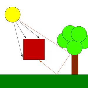
Shadow mapping involves two passes, the first pass renders the scene from te point of view of the light with depth testing enabled and records depth information for each fragment. The resulting depth image (the shadow map) contains depth information for the fragments that are visible from the light source, and therefore, are occluders for any other fragment behind them from the point of view of the light. In other words, these represent the only fragments in the scene that receive direct light, every other fragment is in the shade. In the second pass we render the scene normally to the render target from the point of view of the camera, then for each fragment we need to compute the distance to the light source and compare it against the depth information recorded in the previous pass to decice if the fragment is behind a light occluder or not. If it is, then we remove the diffuse and specular components for the fragment, making it look shadowed.

In this post I will cover the first pass: generation of the shadow map.

Producing the shadow map image

Note: those looking for OpenGL code can have a look at this file ter-shadow-renderer.cpp from my OpenGL terrain renderer demo, which contains the shadow map renderer that generates the shadow map for the sun light in that demo.

Creating a depth image suitable for shadow mapping

The shadow map is a regular depth image were we will record depth information for fragments in light space. This image will be rendered into and sampled from. In Vulkan we can create it like this:

...
VkImageCreateInfo image_info = {};
image_info.sType = VK_STRUCTURE_TYPE_IMAGE_CREATE_INFO;
image_info.pNext = NULL;
image_info.imageType = VK_IMAGE_TYPE_2D;
image_info.format = VK_FORMAT_D32_SFLOAT;
image_info.extent.width = SHADOW_MAP_WIDTH;
image_info.extent.height = SHADOW_MAP_HEIGHT;
image_info.extent.depth = 1;
image_info.mipLevels = 1;
image_info.arrayLayers = 1;
image_info.samples = VK_SAMPLE_COUNT_1_BIT;
image_info.initialLayout = VK_IMAGE_LAYOUT_UNDEFINED;
image_info.usage = VK_IMAGE_USAGE_DEPTH_STENCIL_ATTACHMENT_BIT |
                   VK_IMAGE_USAGE_SAMPLED_BIT;
image_info.queueFamilyIndexCount = 0;
image_info.pQueueFamilyIndices = NULL;
image_info.sharingMode = VK_SHARING_MODE_EXCLUSIVE;
image_info.flags = 0;

VkImage image;
vkCreateImage(device, &image_info, NULL, &image);
...

The code above creates a 2D image with a 32-bit float depth format. The shadow map’s width and height determine the resolution of the depth image: larger sizes produce higher quality shadows but of course this comes with an additional computing cost, so you will probably need to balance quality and performance for your particular target. In the first pass of the algorithm we need to render to this depth image, so we include the VK_IMAGE_USAGE_DEPTH_STENCIL_ATTACHMENT_BIT usage flag, while in the second pass we will sample the shadow map from the fragment shader to decide if each fragment is in the shade or not, so we also include the VK_IMAGE_USAGE_SAMPLED_BIT.

One more tip: when we allocate and bind memory for the image, we probably want to request device local memory too (VK_MEMORY_PROPERTY_DEVICE_LOCAL_BIT) for optimal performance, since we won’t need to map the shadow map memory in the host for anything.

Since we are going to render to this image in the first pass of the process we also need to create a suitable image view that we can use to create a framebuffer. There are no special requirements here, we just create a view with the same format as the image and with a depth aspect:

...
VkImageViewCreateInfo view_info = {};
view_info.sType = VK_STRUCTURE_TYPE_IMAGE_VIEW_CREATE_INFO;
view_info.pNext = NULL;
view_info.image = image;
view_info.format = VK_FORMAT_D32_SFLOAT;
view_info.components.r = VK_COMPONENT_SWIZZLE_R;
view_info.components.g = VK_COMPONENT_SWIZZLE_G;
view_info.components.b = VK_COMPONENT_SWIZZLE_B;
view_info.components.a = VK_COMPONENT_SWIZZLE_A;
view_info.subresourceRange.aspectMask = VK_IMAGE_ASPECT_DEPTH_BIT;
view_info.subresourceRange.baseMipLevel = 0;
view_info.subresourceRange.levelCount = 1;
view_info.subresourceRange.baseArrayLayer = 0;
view_info.subresourceRange.layerCount = 1;
view_info.viewType = VK_IMAGE_VIEW_TYPE_2D;
view_info.flags = 0;

VkImageView shadow_map_view;
vkCreateImageView(device, &view_info, NULL, &view);
...

Rendering the shadow map

In order to generate the shadow map image we need to render the scene from the point of view of the light, so first, we need to compute the corresponding View and Projection matrices. How we calculate these matrices depends on the type of light we are using. As described in the previous post, we can consider 3 types of lights: spotlights, positional lights and directional lights.

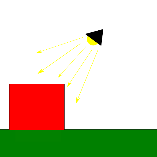
Spotlights are the easiest for shadow mapping, since with these we use regular perspective projection.

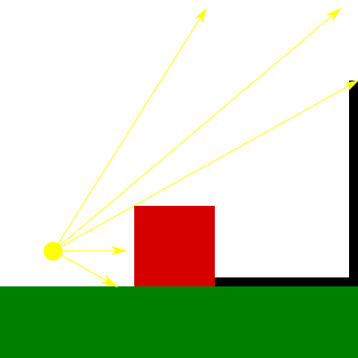
Positional lights work similar to spotlights in the sense that they also use perspective projection, however, because these are omnidirectional, they see the entire scene around them. This means that we need to render a shadow map that contains scene objects in all directions around the light. We can do this by using a cube texture for the shadow map instead of a regular 2D texture and render the scene 6 times adjusting the View matrix to capture scene objects in front of the light, behind it, to its left, to its right, above and below. In this case we want to use a field of view of 45º with the projection matrix so that the set of 6 images captures the full scene around the light source with no image overlaps.

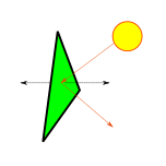
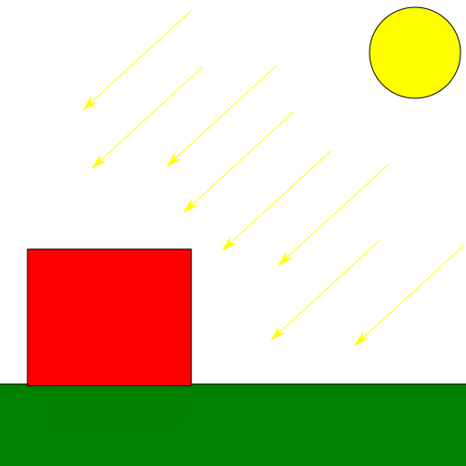
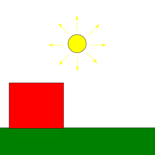
Finally, we have directional lights. In the previous post I mentioned that these lights model light sources which rays are parallel and because of this feature they cast regular shadows (that is, shadows that are not perspective projected). Thus, to render shadow maps for directional lights we want to use orthographic projection instead of perspective projection.

In this post I will focus on creating a shadow map for a spotlight source only. I might write follow up posts in the future covering other light sources, but for the time being, you can have a look at my OpenGL terrain renderer demo if you are interested in directional lights.

So, for a spotlight source, we just define a regular perspective projection, like this:

glm::mat4 clip = glm::mat4(1.0f, 0.0f, 0.0f, 0.0f,
                           0.0f,-1.0f, 0.0f, 0.0f,
                           0.0f, 0.0f, 0.5f, 0.0f,
                           0.0f, 0.0f, 0.5f, 1.0f);

glm::mat4 light_projection = clip *
      glm::perspective(glm::radians(45.0f),
                       (float) SHADOW_MAP_WIDTH / SHADOW_MAP_HEIGHT,
                       LIGHT_NEAR, LIGHT_FAR);

The code above generates a regular perspective projection with a field of view of 45º. We should adjust the light’s near and far planes to make them as tight as possible to reduce artifacts when we use the shadow map to render the shadows in the scene (I will go deeper into this in a later post). In order to do this we should consider that the near plane can be increased to reflect the closest that an object can be to the light (that might depend on the scene, of course) and the far plane can be decreased to match the light’s area of influence (determined by its attenuation factors, as explained in the previous post).

The clip matrix is not specific to shadow mapping, it just makes it so that the resulting projection considers the particularities of how the Vulkan coordinate system is defined (Y axis is inversed, Z range is halved).

As usual, the projection matrix provides us with a projection frustrum, but we still need to point that frustum in the direction in which our spotlight is facing, so we also need to compute the view matrix transform of our spotlight. One way to define the direction in which our spotlight is facing is by having the rotation angles of spotlight on each axis, similarly to what we would do to compute the view matrix of our camera:

glm::mat4
compute_view_matrix_for_rotation(glm::vec3 origin, glm::vec3 rot)
{
   glm::mat4 mat(1.0);
   float rx = DEG_TO_RAD(rot.x);
   float ry = DEG_TO_RAD(rot.y);
   float rz = DEG_TO_RAD(rot.z);
   mat = glm::rotate(mat, -rx, glm::vec3(1, 0, 0));
   mat = glm::rotate(mat, -ry, glm::vec3(0, 1, 0));
   mat = glm::rotate(mat, -rz, glm::vec3(0, 0, 1));
   mat = glm::translate(mat, -origin);
   return mat;
}

Here, origin is the position of the light source in world space, and rot represents the rotation angles of the light source on each axis, representing the direction in which the spotlight is facing.

Now that we have the View and Projection matrices that define our light space we can go on and render the shadow map. For this we need to render scene as we normally would but instead of using our camera’s View and Projection matrices, we use the light’s. Let’s have a look at the shadow map rendering code:

Render pass

static VkRenderPass
create_shadow_map_render_pass(VkDevice device)
{
   VkAttachmentDescription attachments[2];

   // Depth attachment (shadow map)
   attachments[0].format = VK_FORMAT_D32_SFLOAT;
   attachments[0].samples = VK_SAMPLE_COUNT_1_BIT;
   attachments[0].loadOp = VK_ATTACHMENT_LOAD_OP_CLEAR;
   attachments[0].storeOp = VK_ATTACHMENT_STORE_OP_STORE;
   attachments[0].stencilLoadOp = VK_ATTACHMENT_LOAD_OP_DONT_CARE;
   attachments[0].stencilStoreOp = VK_ATTACHMENT_STORE_OP_DONT_CARE;
   attachments[0].initialLayout = VK_IMAGE_LAYOUT_UNDEFINED;
   attachments[0].finalLayout = VK_IMAGE_LAYOUT_SHADER_READ_ONLY_OPTIMAL;
   attachments[0].flags = 0;

   // Attachment references from subpasses
   VkAttachmentReference depth_ref;
   depth_ref.attachment = 0;
   depth_ref.layout = VK_IMAGE_LAYOUT_DEPTH_STENCIL_ATTACHMENT_OPTIMAL;

   // Subpass 0: shadow map rendering
   VkSubpassDescription subpass[1];
   subpass[0].pipelineBindPoint = VK_PIPELINE_BIND_POINT_GRAPHICS;
   subpass[0].flags = 0;
   subpass[0].inputAttachmentCount = 0;
   subpass[0].pInputAttachments = NULL;
   subpass[0].colorAttachmentCount = 0;
   subpass[0].pColorAttachments = NULL;
   subpass[0].pResolveAttachments = NULL;
   subpass[0].pDepthStencilAttachment = &depth_ref;
   subpass[0].preserveAttachmentCount = 0;
   subpass[0].pPreserveAttachments = NULL;

   // Create render pass
   VkRenderPassCreateInfo rp_info;
   rp_info.sType = VK_STRUCTURE_TYPE_RENDER_PASS_CREATE_INFO;
   rp_info.pNext = NULL;
   rp_info.attachmentCount = 1;
   rp_info.pAttachments = attachments;
   rp_info.subpassCount = 1;
   rp_info.pSubpasses = subpass;
   rp_info.dependencyCount = 0;
   rp_info.pDependencies = NULL;
   rp_info.flags = 0;

   VkRenderPass render_pass;
   VK_CHECK(vkCreateRenderPass(device, &rp_info, NULL, &render_pass));

   return render_pass;
}

The render pass is simple enough: we only have one attachment with the depth image and one subpass that renders to the shadow map target. We will start the render pass by clearing the shadow map and by the time we are done we want to store it and transition it to layout VK_IMAGE_LAYOUT_SHADER_READ_ONLY_OPTIMAL so we can sample from it later when we render the scene with shadows. Notice that because we only care about depth information, the render pass doesn’t include any color attachments.

Framebuffer

Every rendering job needs a target framebuffer, so we need to create one for our shadow map. For this we will use the image view we created from the shadow map image. We link this framebuffer target to the shadow map render pass description we have just defined:

VkFramebufferCreateInfo fb_info;
fb_info.sType = VK_STRUCTURE_TYPE_FRAMEBUFFER_CREATE_INFO;
fb_info.pNext = NULL;
fb_info.renderPass = shadow_map_render_pass;
fb_info.attachmentCount = 1;
fb_info.pAttachments = &shadow_map_view;
fb_info.width = SHADOW_MAP_WIDTH;
fb_info.height = SHADOW_MAP_HEIGHT;
fb_info.layers = 1;
fb_info.flags = 0;

VkFramebuffer shadow_map_fb;
vkCreateFramebuffer(device, &fb_info, NULL, &shadow_map_fb);

Pipeline description

The pipeline we use to render the shadow map also has some particularities:

Because we only care about recording depth information, we can typically skip any vertex attributes other than the positions of the vertices in the scene:

...
VkVertexInputBindingDescription vi_binding[1];
VkVertexInputAttributeDescription vi_attribs[1];

// Vertex attribute binding 0, location 0: position
vi_binding[0].binding = 0;
vi_binding[0].inputRate = VK_VERTEX_INPUT_RATE_VERTEX;
vi_binding[0].stride = 2 * sizeof(glm::vec3);

vi_attribs[0].binding = 0;
vi_attribs[0].location = 0;
vi_attribs[0].format = VK_FORMAT_R32G32B32_SFLOAT;
vi_attribs[0].offset = 0;

VkPipelineVertexInputStateCreateInfo vi;
vi.sType = VK_STRUCTURE_TYPE_PIPELINE_VERTEX_INPUT_STATE_CREATE_INFO;
vi.pNext = NULL;
vi.flags = 0;
vi.vertexBindingDescriptionCount = 1;
vi.pVertexBindingDescriptions = vi_binding;
vi.vertexAttributeDescriptionCount = 1;
vi.pVertexAttributeDescriptions = vi_attribs;
...
pipeline_info.pVertexInputState = &vi;
...

The code above defines a single vertex attribute for the position, but assumes that we read this from a vertex buffer that packs interleaved positions and normals for each vertex (each being a vec3) so we use the binding’s stride to jump over the normal values in the buffer. This is because in this particular example, we have a single vertex buffer that we reuse for both shadow map rendering and normal scene rendering (which requires vertex normals for lighting computations).

Again, because we do not produce color data, we can skip the fragment shader and our vertex shader is a simple passthough instead of the normal vertex shader we use with the scene:

....
VkPipelineShaderStageCreateInfo shader_stages[1];
shader_stages[0].sType =
   VK_STRUCTURE_TYPE_PIPELINE_SHADER_STAGE_CREATE_INFO;
shader_stages[0].pNext = NULL;
shader_stages[0].pSpecializationInfo = NULL;
shader_stages[0].flags = 0;
shader_stages[0].stage = VK_SHADER_STAGE_VERTEX_BIT;
shader_stages[0].pName = "main";
shader_stages[0].module = create_shader_module("shadowmap.vert.spv", ...);
...
pipeline_info.pStages = shader_stages;
pipeline_info.stageCount = 1;
...

This is how the shadow map vertex shader (shadowmap.vert) looks like in GLSL:

#version 400

#extension GL_ARB_separate_shader_objects : enable
#extension GL_ARB_shading_language_420pack : enable

layout(std140, set = 0, binding = 0) uniform vp_ubo {
    mat4 ViewProjection;
} VP;

layout(std140, set = 0, binding = 1) uniform m_ubo {
     mat4 Model[16];
} M;

layout(location = 0) in vec3 in_position;

void main()
{
   vec4 pos = vec4(in_position.x, in_position.y, in_position.z, 1.0);
   vec4 world_pos = M.Model[gl_InstanceIndex] * pos;
   gl_Position = VP.ViewProjection * world_pos;
}

The shader takes the ViewProjection matrix of the light (we have already multiplied both together in the host) and a UBO with the Model matrices of each object in the scene as external resources (we use instanced rendering in this particular example) as well as a single vec3 input attribute with the vertex position. The only job of the vertex shader is to compute the position of the vertex in the transformed space (the light space, since we are passing the ViewProjection matrix of the light), nothing else is done here.

Command buffer

The command buffer is pretty similar to the one we use with the scene, only that we render to the shadow map image instead of the usual render target. In the shadow map render pass description we have indicated that we will clear it, so we need to include a depth clear value. We also need to make sure that we set the viewport and sccissor to match the shadow map dimensions:

...
VkClearValue clear_values[1];
clear_values[0].depthStencil.depth = 1.0f;
clear_values[0].depthStencil.stencil = 0;

VkRenderPassBeginInfo rp_begin;
rp_begin.sType = VK_STRUCTURE_TYPE_RENDER_PASS_BEGIN_INFO;
rp_begin.pNext = NULL;
rp_begin.renderPass = shadow_map_render_pass;
rp_begin.framebuffer = shadow_map_framebuffer;
rp_begin.renderArea.offset.x = 0;
rp_begin.renderArea.offset.y = 0;
rp_begin.renderArea.extent.width = SHADOW_MAP_WIDTH;
rp_begin.renderArea.extent.height = SHADOW_MAP_HEIGHT;
rp_begin.clearValueCount = 1;
rp_begin.pClearValues = clear_values;

vkCmdBeginRenderPass(shadow_map_cmd_buf,
                     &rp_begin,
                     VK_SUBPASS_CONTENTS_INLINE);

VkViewport viewport;
viewport.height = SHADOW_MAP_HEIGHT;
viewport.width = SHADOW_MAP_WIDTH;
viewport.minDepth = 0.0f;
viewport.maxDepth = 1.0f;
viewport.x = 0;
viewport.y = 0;
vkCmdSetViewport(shadow_map_cmd_buf, 0, 1, &viewport);

VkRect2D scissor;
scissor.extent.width = SHADOW_MAP_WIDTH;
scissor.extent.height = SHADOW_MAP_HEIGHT;
scissor.offset.x = 0;
scissor.offset.y = 0;
vkCmdSetScissor(shadow_map_cmd_buf, 0, 1, &scissor);
...

Next, we bind the shadow map pipeline we created above, bind the vertex buffer and descriptor sets as usual and draw the scene geometry.

...
vkCmdBindPipeline(shadow_map_cmd_buf,
                  VK_PIPELINE_BIND_POINT_GRAPHICS,
                  shadow_map_pipeline);

const VkDeviceSize offsets[1] = { 0 };
vkCmdBindVertexBuffers(shadow_cmd_buf, 0, 1, vertex_buf, offsets);

vkCmdBindDescriptorSets(shadow_map_cmd_buf,
                        VK_PIPELINE_BIND_POINT_GRAPHICS,
                        shadow_map_pipeline_layout,
                        0, 1,
                        shadow_map_descriptor_set,
                        0, NULL);

vkCmdDraw(shadow_map_cmd_buf, ...);

vkCmdEndRenderPass(shadow_map_cmd_buf);
...

Notice that the shadow map pipeline layout will be different from the one used with the scene too. Specifically, during scene rendering we will at least need to bind the shadow map for sampling and we will probably also bind additional resources to access light information, surface materials, etc that we don’t need to render the shadow map, where we only need the View and Projection matrices of the light plus the UBO with the model matrices of the objects in the scene.

We are almost there, now we only need to submit the command buffer for execution to render the shadow map:

...
VkPipelineStageFlags shadow_map_wait_stages = 0;
VkSubmitInfo submit_info = { };
submit_info.pNext = NULL;
submit_info.sType = VK_STRUCTURE_TYPE_SUBMIT_INFO;
submit_info.waitSemaphoreCount = 0;
submit_info.pWaitSemaphores = NULL;
submit_info.signalSemaphoreCount = 1;
submit_info.pSignalSemaphores = &signal_sem;
submit_info.pWaitDstStageMask = 0;
submit_info.commandBufferCount = 1;
submit_info.pCommandBuffers = &shadow_map_cmd_buf;

vkQueueSubmit(queue, 1, &submit_info, NULL);
...

Because the next pass of the algorithm will need to sample the shadow map during the final scene rendering,we use a semaphore to ensure that we complete this work before we start using it in the next pass of the algorithm.

In most scenarios, we will want to render the shadow map on every frame to account for dynamic objects that move in the area of effect of the light or even moving lights, however, if we can ensure that no objects have altered their positions inside the area of effect of the light and that the light’s description (position/direction) hasn’t changed, we may not need need to regenerate the shadow map and save some precious rendering time.

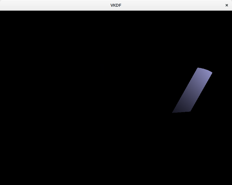
Visualizing the shadow map

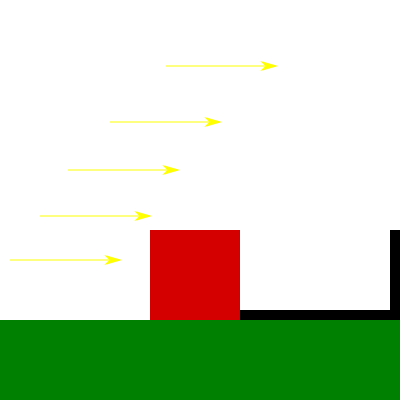
After executing the shadow map rendering job our shadow map image contains the depth information of the scene from the point of view of the light. Before we go on and start using this as input to produce shadows in our scene, we should probably try to visualize the shadow map to verify that it is correct. For this we just need to submit a follow-up job that takes the shadow map image as a texture input and renders it to a quad on the screen. There is one caveat though: when we use perspective projection, Z values in the depth buffer are not linear, instead precission is larger at distances closer to the near plane and drops as we get closer to the far place in order to improve accuracy in areas closer to the observer and avoid Z-fighting artifacts. This means that we probably want to linearize our shadow map values when we sample from the texture so that we can actually see things, otherwise most things that are not close enough to the light source will be barely visible:

#version 400

#extension GL_ARB_separate_shader_objects : enable
#extension GL_ARB_shading_language_420pack : enable

layout(std140, set = 0, binding = 0) uniform mvp_ubo {
    mat4 mvp;
} MVP;

layout(location = 0) in vec2 in_pos;
layout(location = 1) in vec2 in_uv;

layout(location = 0) out vec2 out_uv;

void main()
{
   gl_Position = MVP.mvp * vec4(in_pos.x, in_pos.y, 0.0, 1.0);
   out_uv = in_uv;
}

#version 400

#extension GL_ARB_separate_shader_objects : enable
#extension GL_ARB_shading_language_420pack : enable

layout (set = 1, binding = 0) uniform sampler2D image;

layout(location = 0) in vec2 in_uv;

layout(location = 0) out vec4 out_color;

void main()
{
   float depth = texture(image, in_uv).r;
   out_color = vec4(1.0 - (1.0 - depth) * 100.0);
}

We can use the vertex and fragment shaders above to render the contents of the shadow map image on to a quad. The vertex shader takes the quad’s vertex positions and texture coordinates as attributes and passes them to the fragment shader, while the fragment shader samples the shadow map at the provided texture coordinates and then “linearizes” the depth value so that we can see better. The code in the shader doesn’t properly linearize the depth values we read from the shadow map (that requires to pass the Z-near and Z-far values used in the projection), but for debugging purposes this works well enough for me, if you use different Z clipping planes you may need to alter the ‘100.0’ value to get good results (or you might as well do a proper conversion considering your actual Z-near and Z-far values).

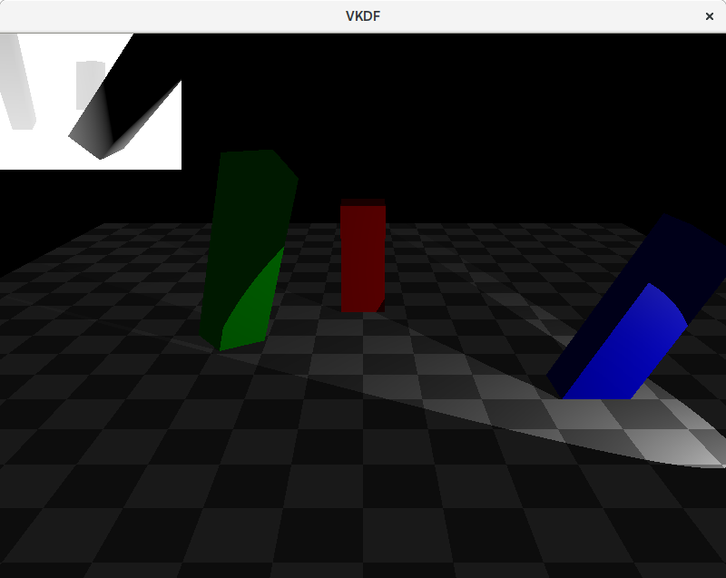
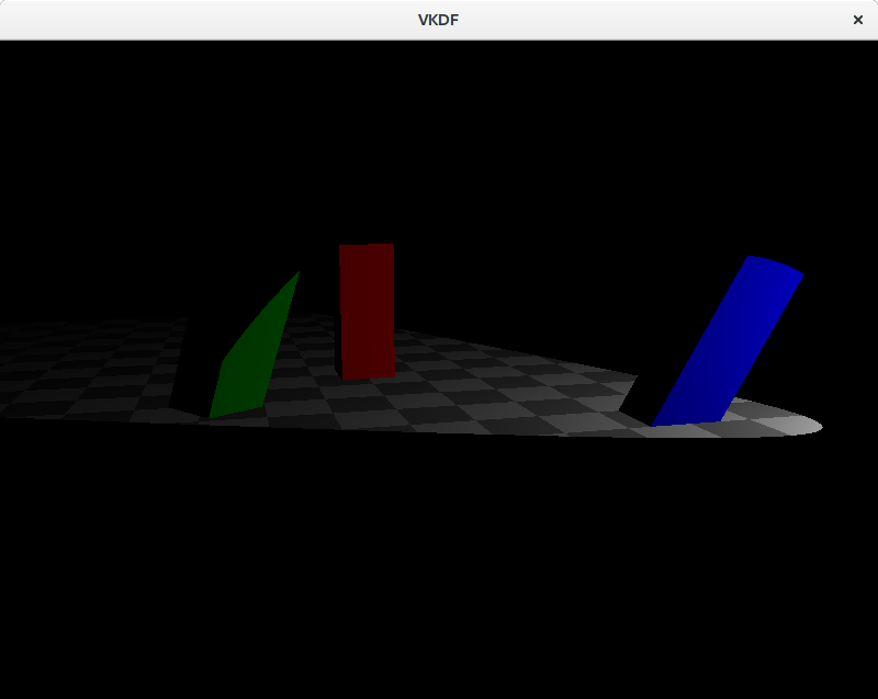
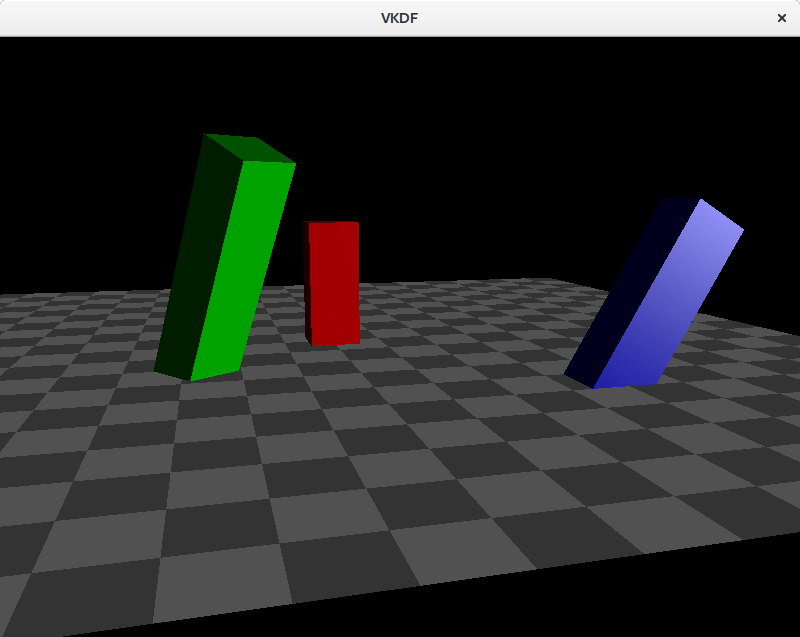
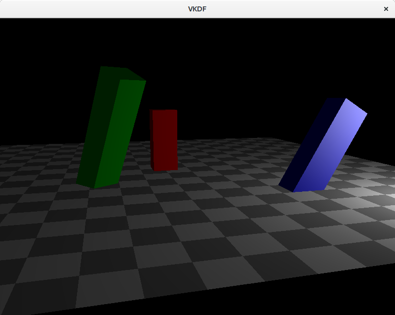
The image shows the shadow map on top of the scene. Darker colors represent smaller depth values, so these are fragments closer to the light source. Notice that we are not rendering the floor geometry to the shadow map since it can’t cast shadows on any other objects in the scene.

Conclusions

In this post we have described the shadow mapping technique as a combination of two passes: the first pass renders a depth image (the shadow map) with the scene geometry from the point of view of the light source. To achieve this, we need a passthrough vertex shader that only transforms the scene vertex positions (using the view and projection transforms from the light) and we can skip the fragment shader completely since we do not care for color output. The second pass, which we will cover in the next post, takes the shadow map as input and uses it to render shadows in the final scene.

Some time ago I promised to write a bit more about how shadow mapping works. It has taken me a while to bring myself to actually deliver on that front, but I have finally decided to put together some posts on this topic, this being the first one. However, before we cover shadow mapping itself we need to cover some lighting basics first. After all, without light there can’t be shadows, right?

This post will introdcuce the popular Phong reflection model as the basis for our lighting model. A lighting model provides a simplified representation of how light works in the natural world that allows us to simulate light in virtual scenes at reasonable computing costs. So let’s dive into it:

Light in the natural world

In the real world, the light that reaches an object is a combination of both direct and indirect light. Direct light is that which comes straight from a light source, while indirect light is the result of light rays hitting other surfaces in the scene, bouncing off of them and eventually reaching the object as a result, maybe after multiple reflections from other objects. Because each time a ray of light hits a surface it loses part of its energy, indirect light reflection is less bright than direct light reflection and its color might have been altered. The contrast between surfaces that are directly hit by the light source and surfaces that only receive indirect light is what creates shadows. A shadow isn’t but the part of a scene that doesn’t receive direct light but might still receive some amount of (less intense) indirect light.

Light in the digital world

Unfortunately, implementing realistic light behavior like that is too expensive, specially for real-time applications, so instead we use simplifications that can produce similar results with much lower computing requirements. The Phong reflection model in particular describes the light reflected from surfaces or emitted by light sources as the combination of 3 components: diffuse, ambient and specular. The model also requires information about the direction in which a particular surface is facing, provided via vectors called surface normals. Let’s introduce each of these concepts:

Surface normals

When we study the behavior of light, we notice that the direction in which surfaces reflect incoming light affects our perception of the surface. For example, if we lit a shiny surface (such as a piece of metal) using a strong light shource so that incoming light is reflected off the surface in the exact opposite direction in which we are looking at it, we will see a strong reflection in the form of highlights. If we move around so that we look at the same surface from a different angle, then we will see the reflection get dimmer and the highlights will eventually disappear. In order to model this behavior we need to know the direction in which the surfaces we render reflect incoming light. The way to do this is by associating vectors called normals with the surfaces we render so that shaders can use that information to produce lighting calculations akin to what we see in the natural world.

Usually, modeling programs can compute normal vectors for us, even model loading libraries can do this work automatically, but some times, for example when we define vertex meshes programatically, we need to define them manually. I won’t covere here how to do this in the general, you can see this article from Khronos if you’re interested in specific algorithms, but I’ll point out something relevant: given a plane, we can compute normal vectors in two opposite directions, one is correct for the front face of the plane/polygon and the other one is correct for the back face, so make sure that if you compute normals manually, you use the correct direction for each face, otherwise you won’t be reflecting light in the correct direction and results won’t be as you expect.

In most scenarios, we only render the front faces of the polygons (by enabling back face culling) and thus, we only care about one of the normal vectors (the one for the front face).

Another thing to notice about normal vectors is that they need to be transformed with the model to be correct for transformed models: if we rotate a model we need to rotate the normals too, since the faces they represent are now rotated and thus, their normal directions have rotated too. Scaling also affects normals, specifically if we don’t use regular scaling, since in that case the orientation of the surfaces may change and affect the direction of the normal vector. Because normal vectors represent directions, their position in world space is irrelevant, so for the purpose of lighting calculations, a normal vector such as (1, 0, 0) defined for a surface placed at (0, 0, 0) is still valid to represent the same surface at any other position in the world; in other words, we do not need to apply translation transforms to our normal vectors.

In practice, the above means that we want to apply the rotation and scale transforms from our models to their normal vectors, but we can skip the translation transform. The matrix representing these transforms is usually called the normal matrix. We can compute the normal matrix from our model matrix by computing the transpose of the inverse of the 3×3 submatrix of the model matrix. Usually, we’d want to compute this matrix in the application and feed it to our vertex shader like we do with our model matrix, but for reference, here is how this can be achieved in the shader code itself, plus how to use this matrix to transform the original normal vectors:

mat3 NormalMatrix = transpose(inverse(mat3(ModelMatrix)));
vec3 out_normal = normalize(NormalMatrix * in_normal);

Notice that the code above normalizes the resulting normal before it is fed to the fragment shader. This is important because the rasterizer will compute normals for all fragments in the surface automatically, and for that it will interpolate between the normals for each vertex we emit. For the interpolated normals to be correct, all vertex normals we output in the vertex shader must have the same length, otherwise the larger normals will deviate the direction of the interpolated vectors towards them because their larger size will increase their weight in the interpolation computations.

Finally, even if we emit normalized vectors in the vertex shader stage, we should note that the interpolated vectors that arrive to the fragment shader are not guaranteed to be normalized. Think for example of the normal vectors (1, 0, 0) and (0, 1, 0) being assigned to the two vertices in a line primitive. At the half-way point in between these two vertices, the interpolator will compute a normal vector of (0.5, 0.5, 0), which is not unit-sized. This means that in the general case, input normals in the fragment shader will need to be normalized again even if have normalized vertex normals at the vertex shader stage.

Diffuse reflection

The diffuse component represents the reflection produced from direct light. It is important to notice that the intensity of the diffuse reflection is affected by the angle between the light coming from the source and the normal of the surface that receives the light. This makes a surface looking straight at the light source be the brightest, with reflection intensity dropping as the angle increases:

In order to compute the diffuse component for a fragment we need its normal vector (the direction in which the surface is facing), the vector from the fragment’s position to the light source, the diffuse component of the light and the diffuse reflection of the fragment’s material:

vec3 normal = normalize(surface_normal);
vec3 pos_to_light_norm = normalize(pos_to_light);
float dp_reflection = max(0.0, dot(normal, pos_to_light_norm));
vec3 diffuse = material.diffuse * light.diffuse * dp_reflection;

Basically, we multiply the diffuse component of the incoming light with the diffuse reflection of the fragment’s material to produce the diffuse component of the light reflected by the fragment. The diffuse component of the surface tells how the object absorbs and reflects incoming light. For example, a pure yellow object (diffuse material vec3(1,1,0)) would absorb the blue component and reflect 100% of the red and green components of the incoming light. If the light is a pure white light (diffuse vec3(1,1,1)), then the observer would see a yellow object. However, if we are using a red light instead (diffuse vec3(1,0,0)), then the light reflected from the surface of the object would only contain the red component (since the light isn’t emitting a green component at all) and we would see it red.

As we said before though, the intensity of the reflection depends on the angle between the incoming light and the direction of the reflection. We account for this with the dot product between the normal at the fragment (surface_normal) and the direction of the light (or rather, the vector pointing from the fragment to the light source). Notice that because the vectors that we use to compute the dot product are normalized, dp_reflection is exactly the cosine of the angle between these two vectors. At an angle of 0º the surface is facing straight at the light source, and the intensity of the diffuse reflection is at its peak, since cosine(0º)=1. At an angle of 90º (or larger) the cosine will be 0 or smaller and will be clamped to 0, meaning that no light is effectively being reflected by the surface (the computed diffuse component will be 0).

Ambient reflection

Computing all possible reflections and bounces of all rays of light from each light source in a scene is way too expensive. Instead, the Phong model approximates this by making indirect reflection from a light source constant across the scene. In other words: it assumes that the amount of indirect light received by any surface in the scene is the same. This eliminates all the complexity while still producing reasonable results in most scenarios. We call this constant factor ambient light.

Adding ambient light to the fragment is then as simple as multiplying the light source’s ambient light by the material’s ambient reflection. The meaning of this product is exactly the same as in the case of the diffuse light, only that it affects the indirect light received by the fragment:

vec3 ambient = material.ambient * light.ambient;

Specular reflection

Very sharp, smooth surfaces such as metal are known to produce specular highlights, which are those bright spots that we can see on shiny objects. Specular reflection depends on the angle between the observer’s view direction and the direction in which the light is reflected off the surface. Specifically, the specular reflection is strongest when the observer is facing exactly in the opposite direction in which the light is reflected. Depending on the properties of the surface, the specular reflection can be more or less focused, affecting how the specular component scatters after being reflected. This property of the material is usually referred to as its shininess.

Implementing specular reflection requires a bit more of work:

vec3 specular = vec3(0);
vec3 light_dir_norm = normalize(vec3(light.direction));
if (dot(normal, -light_dir_norm) >= 0.0) {
   vec3 reflection_dir = reflect(light_dir_norm, normal);
   float shine_factor = dot(reflection_dir, normalize(in_view_dir));
   specular = light.specular.xyz * material.specular.xyz *
         pow(max(0.0, shine_factor), material.shininess.x);
}

Basically, the code above checks if there is any specular reflection at all by computing the cosine of the angle between the fragment’s normal and the direction of the light (notice that, once again, both vectors are normalized prio to using them in the call to dot()). If there is specular reflection, then we compute how shiny the reflection is perceived by the viewer based on the angle between the vector from this fragment to the observer (in_view_dir) and the direction of the light reflected off the fragment’s surface (reflection_dir). The smaller the angle, the more parallel the directions are, meaning that the camera is receiving more reflection and the specular component received is stronger. Finally, we modulate the result based on the shininess of the fragment. We can compute in_view_dir in the vertex shader using the inverse of the View matrix like this:

mat4 ViewInv = inverse(View);
out_view_dir =
   normalize(vec3(ViewInv * vec4(0.0, 0.0, 0.0, 1.0) - world_pos));

The code above takes advantage of the fact that camera transformations are an illusion created by applying the transforms to everything else we render. For example, if we want to create the illusion that the camera is moving to the right, we just apply a translation to everything we render so they show up a bit to the left. This is what our View matrix achieves. From the point of view of GL or Vulkan, the camera is always fixed at (0,0,0). Taking advantage of this, we can compute the position of the virtual observer (the camera) in world space coordinates by applying the inverse of our camera transform to its fixed location (0,0,0). This is what the code above does, where world_pos is the position of this vertex in world space and View is the camera’s view matrix.

In order to produce the final look of the scene according to the Phong reflection model, we need to compute these 3 components for each fragment and add them together:

out_color  = vec4(diffuse + ambient + specular, 1.0)

Attenuation

In most scenarios, light intensity isn’t constant across the scene. Instead, it is brightest at its source and gets dimmer with distance. We can easily model this by adding an attenuation factor that is multiplied by the distance from the fragment to the light source. Typically, the intensity of the light decreases quite fast with distance, so a linear attenuation factor alone may not produce the best results and a quadratic function is preferred:

float attenuation = 1.0 /
    (light.attenuation.constant +
     light.attenuation.linear * dist +
     light.attenuation.quadratic * dist * dist);

diffuse = diffuse * attenuation;
ambient = ambient * attenuation;
specular = specular * attenuation;

Of course, we may decide not to apply attenuation to the ambient component at all if we really want to make it look like it is constant across the scene, however, do notice that when multiple light sources are present, the ambient factors from each source will accumulate and may produce too much ambient light unless they are attenuated.

Types of lights

When we model a light source we also need to consider the kind of light we are manipulating:

Directional lights

These are light sources that emit rays that travel along a specific direction so that all are parallel to each other. We typically use this model to represent bright, distant light sources that produce constant light across the scene. An example would be the sun light. Because the distance to the light source is so large compared to distances in the scene, the attenuation factor is irrelevant and can be discarded. Another particularity of directional light sources is that because the light rays are parallel, shadows casted from them are regular (we will talk more about this once we cover shadow mapping in future posts).

If we had used a directional light in the scene, it would look like this:

Notice how the brightness of the scene doesn’t lower with the distance to the light source.

Point lights

These are light sources for which light originates at a specific position and spreads outwards in all directions. Shadows casted by point lights are not regular, instead they are projected. An example would be the light produced by a light bulb. The attenuation code I showed above would be appropriate to represent point lights.

Here is how the scene would look like with a point light:

In this case, we can see how attenuation plays a factor and brightness lowers as we walk away from the light source (which is close to the blue cuboid).

Spotlights

This is the light source I used to illustrate the diffuse, ambient and specular components. They are similar to point lights, is the sense that light originates from a specific point in space and spreads outwards, however, instead of scattering in all directions, rays scatter forming a cone with the tip at the origin of the light. The angle formed by the lights’s direction and the sides of the cone is usually called the cutoff angle, because not light is casted outside its limits. Flashlights are a good example of this type of light.

In order to create spotlights we need to consider the cutoff angle of the light and make sure that no diffuse or specular component is reflected by a fragment which is beyond the cutoff threshold:

vec3 light_to_pos_norm = -pos_to_light_norm;
float dp = dot(light_to_pos_norm, light_dir_norm);
if (dp <= light.cutoff) {
   diffuse = vec3(0);
   specular = vec3(0);
}

In the code above we compute the cosine of the angle between the light’s direction and the vector from the light to the fragment (dp). Here, light.cutoff represents the cosine of the spotlight’s cutoff angle too, so when dp is smaller it means that the fragment is outside the light cone emitted by the spotlight and we remove its diffuse and specular reflections completely.

Multiple lights

Handling multiple lights is easy enough: we only need to compute the color contribution for each light separately and then add all of them together for each fragment (pseudocode):

vec3 fragColor = vec3(0);
foreach light in lights
    fragColor += compute_color_for_light(light, ...);
...

Of course, light attenuation plays a vital role here to limit the area of influence of each light so that scenes where we have multiple lights don’t get too bright.

An important thing to notice above the pseudocode above is that this process involves looping through costy per-fragment light computations for each light source, which can lead to important performance hits as the number of lights in the scene increases. This shading model, as described here, is called forward rendering and it has the benefit that it is very simple to implement but its downside is that we may incur in many costy lighting computations for fragments that, eventually, won’t be visible in the screen (due to them being occluded by other fragments). This is particularly important when the number of lights in the scene is quite large and its complexity makes it so that there are many occluded fragments. Another technique that may be more suitable for these situations is called deferred rendering, which postpones costy shader computations to a later stage (hence the word deferred) in which we only evaluate them for fragments that are known to be visible, but that is a topic for another day, in this series we will focus on forward rendering only.

Lights and shadows

For the purpose of shadow mapping in particular we should note that objects that are directly lit by the light source reflect all 3 of the light components, while objects in the shadow only reflect the ambient component. Because objects that only reflect ambient light are less bright, they appear shadowed, in similar fashion as they would in the real world. We will see the details how this is done in the next post, but for the time being, keep this in mind.

Source code

The scene images in this post were obtained from a simple shadow mapping demo I wrote in Vulkan. The source code for that is available here, and it includes also the shadow mapping implementation that I’ll cover in the next post. Specifically relevant to this post are the scene vertex and fragment shaders where lighting calculations take place.

Conclusions

In order to represent shadows we first need a means to represent light. In this post we discussed the Phong reflection model as a simple, yet effective way to model light reflection in a scene as the addition of three separate components: diffuse, ambient and specular. Once we have a representation of light we can start discussing shadows, which are parts of the scene that only receive ambient light because other objects occlude the diffuse and specular components of the light source.