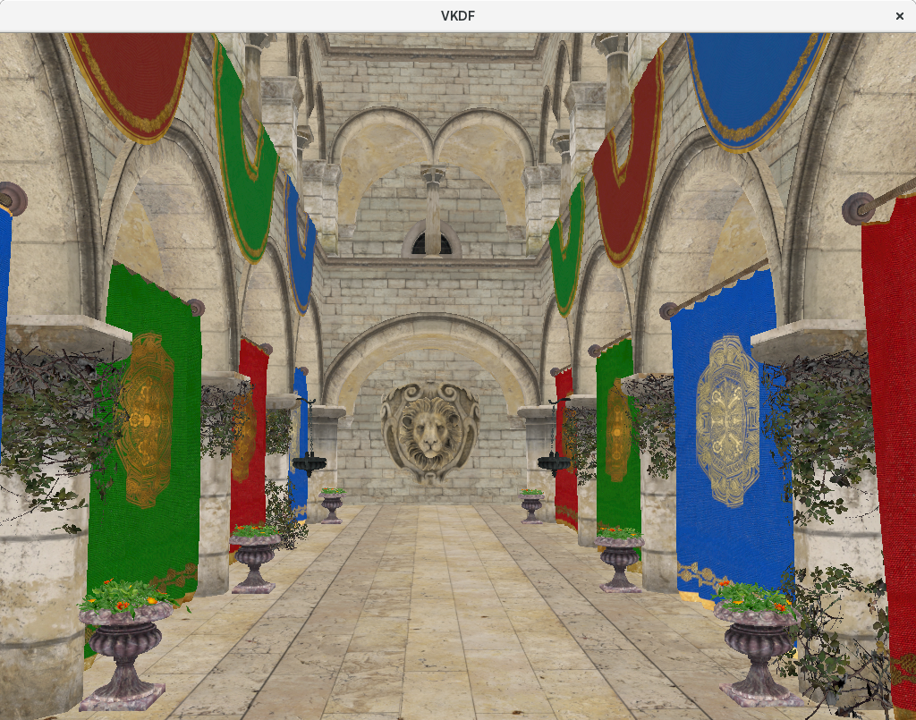
For some time now I have been working on a personal project to render the well known Sponza model provided by Crytek using Vulkan. Here is a picture of the current (still a work-in-progress) result:
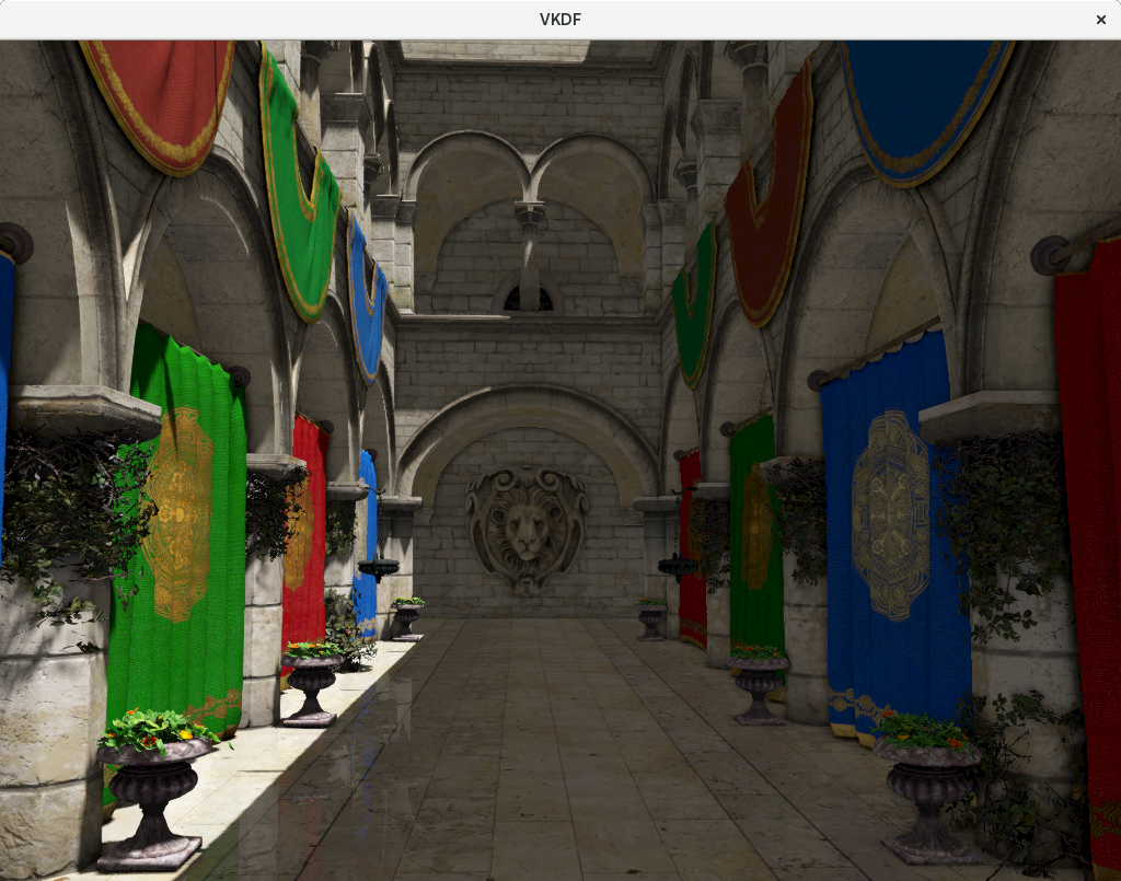
This screenshot was captured on my Intel Kabylake laptop, running on the Intel Mesa Vulkan driver (Anvil).
The following list includes the main features implemented in the demo:
- Depth pre-pass
- Forward and deferred rendering paths
- Anisotropic filtering
- Shadow mapping with Percentage-Closer Filtering
- Bump mapping
- Screen Space Ambient Occlusion (only on the deferred path)
- Screen Space Reflections (only on the deferred path)
- Tone mapping
- Anti-aliasing (FXAA)
I have been thinking about writing post about this for some time, but given that there are multiple features involved I wasn’t sure how to scope it. Eventually I decided to write a “frame analysis” post where I describe, step by step, all the render passes involved in the production of the single frame capture showed at the top of the post. I always enjoyed reading this kind of articles so I figured it would be fun to write one myself and I hope others find it informative, if not entertaining.
To avoid making the post too dense I won’t go into too much detail while describing each render pass, so don’t expect me to go into the nitty-gritty of how I implemented Screen Space Ambient Occlussion for example. Instead I intend to give a high-level overview of how the various features implemented in the demo work together to create the final result. I will provide screenshots so that readers can appreciate the outputs of each step and verify how detail and quality build up over time as we include more features in the pipeline. Those who are more interested in the programming details of particular features can always have a look at the Vulkan source code (link available at the bottom of the article), look for specific tutorials available on the Internet or wait for me to write feature-specifc posts (I don’t make any promises though!).
If you’re interested in going through with this then grab a cup of coffe and get ready, it is going to be a long ride!
Step 0: Culling
This is the only step in this discussion that runs on the CPU, and while optional from the point of view of the result (it doesn’t affect the actual result of the rendering), it is relevant from a performance point of view. Prior to rendering anything, in every frame, we usually want to cull meshes that are not visible to the camera. This can greatly help performance, even on a relatively simple scene such as this. This is of course more noticeable when the camera is looking in a direction in which a significant amount of geometry is not visible to it, but in general, there are always parts of the scene that are not visible to the camera, so culling is usually going to give you a performance bonus.
In large, complex scenes with tons of objects we probably want to use more sophisticated culling methods such as Quadtrees, but in this case, since the number of meshes is not too high (the Sponza model is slightly shy of 400 meshes), we just go though all of them and cull them individually against the camera’s frustum, which determines the area of the 3D space that is visible to the camera.
The way culling works is simple: for each mesh we compute an axis-aligned bounding box and we test that box for intersection with the camera’s frustum. If we can determine that the box never intersects, then the mesh enclosed within it is not visible and we flag it as such. Later on, at rendering time (or rather, at command recording time, since the demo has been written in Vulkan) we just skip the meshes that have been flagged.
The algorithm is not perfect, since it is possible that an axis-aligned bounding box for a particular mesh is visible to the camera and yet no part of the mesh itself is visible, but it should not affect a lot of meshes and trying to improve this would incur in additional checks that could undermine the efficiency of the process anyway.
Since in this particular demo we only have static geometry we only need to run the culling pass when the camera moves around, since otherwise the list of visible meshes doesn’t change. If dynamic geometry were present, we would need to at least cull dynamic geometry on every frame even if the camera stayed static, since dynamic elements may step in (or out of) the viewing frustum at any moment.
Step 1: Depth pre-pass
This is an optional stage, but it can help performance significantly in many cases. The idea is the following: our GPU performance is usually going to be limited by the fragment shader, and very specially so as we target higher resolutions. In this context, without a depth pre-pass, we are very likely going to execute the fragment shader for fragments that will not end up in the screen because they are occluded by fragments produced by other geometry in the scene that will be rasterized to the same XY screen-space coordinates but with a smaller Z coordinate (closer to the camera). This wastes precious GPU resources.
One way to improve the situation is to sort our geometry by distance from the camera and render front to back. With this we can get fragments that are rasterized from background geometry quickly discarded by early depth tests before the fragment shader runs for them. Unfortunately, although this will certainly help (assuming we can spare the extra CPU work to keep our geometry sorted for every frame), it won’t eliminate all the instances of the problem in the general case.
Also, some times things are more complicated, as the shading cost of different pieces of geometry can be very different and we should also take this into account. For example, we can have a very large piece of geometry for which some pixels are very close to the camera while some others are very far away and that has a very expensive shader. If our renderer is doing front-to-back rendering without any other considerations it will likely render this geometry early (since parts of it are very close to the camera), which means that it will shade all or most of its very expensive fragments. However, if the renderer accounts for the relative cost of the shader execution it would probably postpone rendering it as much as possible, so by the time it actually renders it, it takes advantage of early fragment depth tests to avoid as many of its expensive fragment shader executions as possible.
Using a depth-prepass ensures that we only run our fragment shader for visible fragments, and only those, no matter the situation. The downside is that we have to execute a separate rendering pass where we render our geometry to the depth buffer so that we can identify the visible fragments. This pass is usually very fast though, since we don’t even need a fragment shader and we are only writing to a depth texture. The exception to this rule is geometry that has opacity information, such as opacity textures, in which case we need to run a cheap fragment shader to identify transparent pixels and discard them so they don’t hit the depth buffer. In the Sponza model we need to do that for the flowers or the vines on the columns for example.
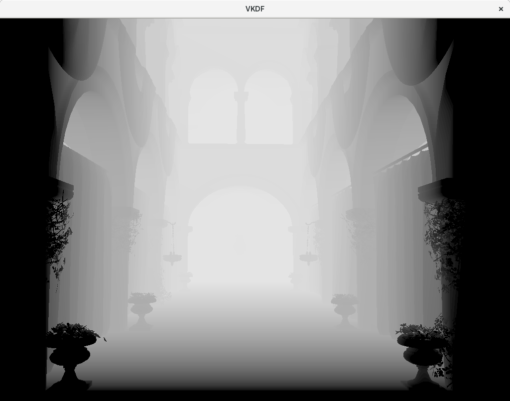
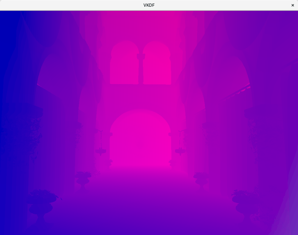
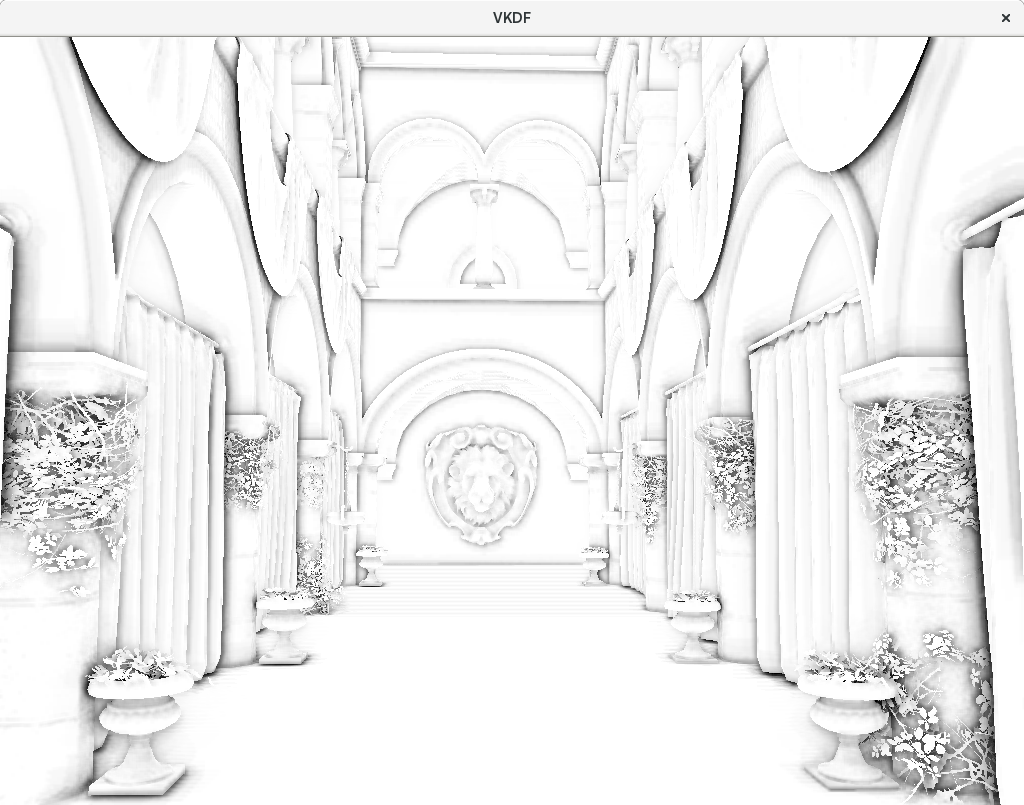
The picture shows the output of the depth pre-pass. Darker colors mean smaller distance from the camera. That’s why the picture gets brighter as we move further away.
Now, the remaining passes will be able to use this information to limit their shading to fragments that, for a given XY screen-space position, match exactly the Z value stored in the depth buffer, effectively selecting only the fragments that will be visible in the screen. We do this by configuring the depth test to do an EQUAL test instead of the usual LESS test, which is what we use in the depth-prepass.
In this particular demo, running on my Intel GPU, the depth pre-pass is by far the cheapest of all the GPU passes and it definitely pays off in terms of overall performance output.
Step 2: Shadow map
In this demo we have single source of light produced by a directional light that simulates the sun. You can probably guess the direction of the light by checking out the picture at the top of this post and looking at the direction projected shadows.
I already covered how shadow mapping works in previous series of posts, so if you’re interested in the programming details I encourage you to read that. Anyway, the basic idea is that we want to capture the scene from the point of view of the light source (to be more precise, we want to capture the objects in the scene that can potentially produce shadows that are visible to our camera).
With that information, we will be able to inform out lighting pass so it can tell if a particular fragment is in the shadows (not visible from our light’s perspective) or in the light (visible from our light’s perspective) and shade it accordingly.
From a technical point of view, recording a shadow map is exactly the same as the depth-prepass: we basically do a depth-only rendering and capture the result in a depth texture. The main differences here are that we need to render from the point of view of the light instead of our camera’s and that this being a directional light, we need to use an orthographic projection and adjust it properly so we capture all relevant shadow casters around the camera.
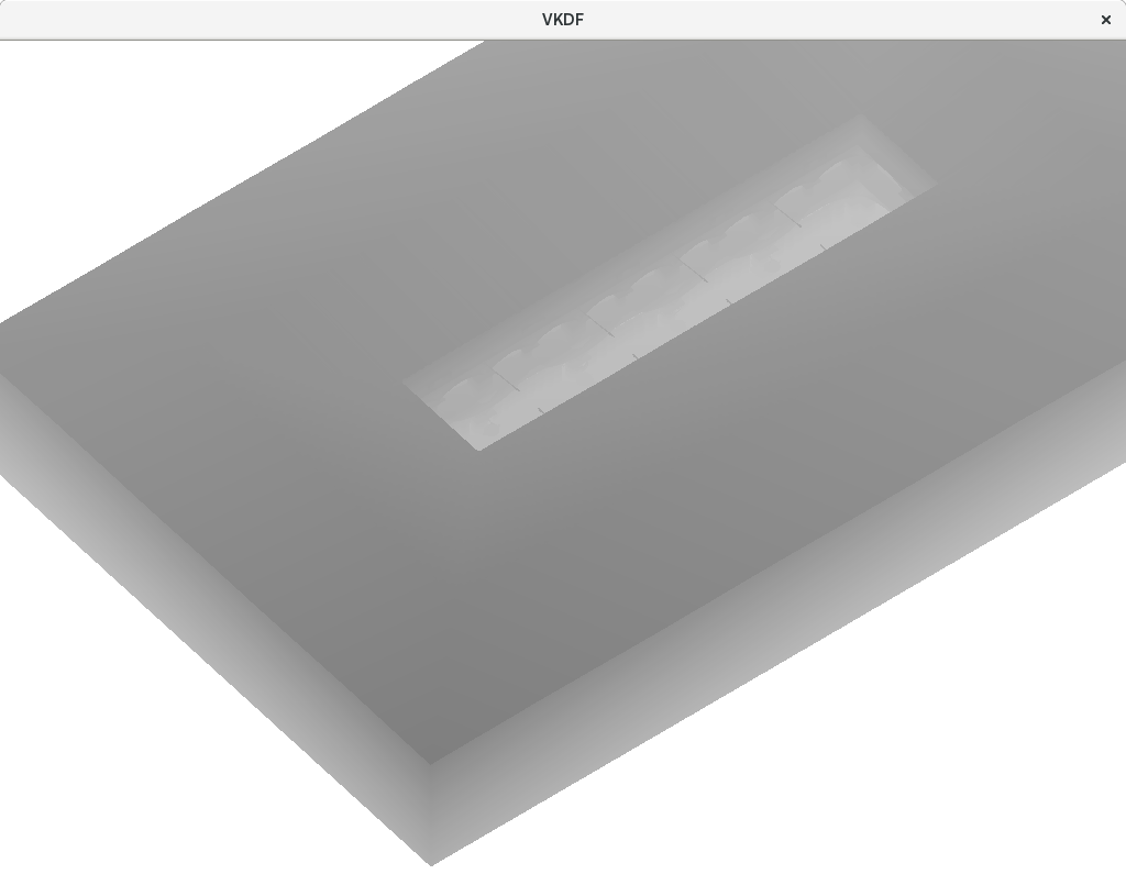
In the image above we can see the shadow map generated for this frame. Again, the brighter the color, the further away the fragment is from the light source. The bright white area outside the atrium building represents the part of the scene that is empty and thus ends with the maximum depth, which is what we use to clear the shadow map before rendering to it.
In this case, we are using a 4096×4096 texture to store the shadow map image, much larger than our rendering target. This is because shadow mapping from directional lights needs a lot of precision to produce good results, otherwise we end up with very pixelated / blocky shadows, more artifacts and even missing shadows for small geometry. To illustrate this better here is the same rendering of the Sponza model from the top of this post, but using a 1024×1024 shadow map (floor reflections are disabled, but that is irrelevant to shadow mapping):
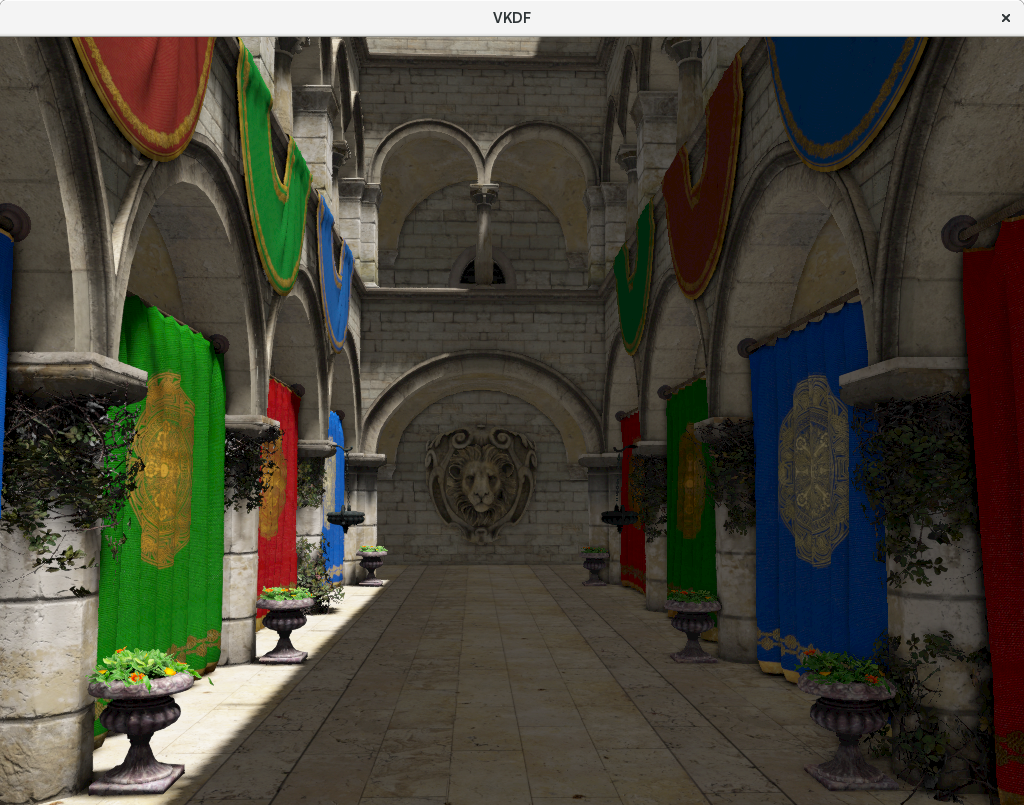
You can see how in the 1024×1024 version there are some missing shadows for the vines on the columns and generally blurrier shadows (when not also slightly distorted) everywhere else.
Step 3: GBuffer
In deferred rendering we capture various attributes of the fragments produced by rasterizing our geometry and write them to separate textures that we will use to inform the lighting pass later on (and possibly other passes).
What we do here is to render our geometry normally, like we did in our depth-prepass, but this time, as we explained before, we configure the depth test to only pass fragments that match the contents of the depth-buffer that we produced in the depth-prepass, so we only process fragments that we now will be visible on the screen.
Deferred rendering uses multiple render targets to capture each of these attributes to a different texture for each rasterized fragment that passes the depth test. In this particular demo our GBuffer captures:
- Normal vector
- Diffuse color
- Specular color
- Position of the fragment from the point of view of the light (for shadow mapping)
It is important to be very careful when defining what we store in the GBuffer: since we are rendering to multiple screen-sized textures, this pass has serious bandwidth requirements and therefore, we should use texture formats that give us the range and precision we need with the smallest pixel size requirements and avoid storing information that we can get or compute efficiently through other means. This is particularly relevant for integrated GPUs that don’t have dedicated video memory (such as my Intel GPU).
In the demo, I do lighting in view-space (that is the coordinate space used takes the camera as its origin), so I need to work with positions and vectors in this coordinate space. One of the parameters we need for lighting is surface normals, which are conveniently stored in the GBuffer, but we will also need to know the view-space position of the fragments in the screen. To avoid storing the latter in the GBuffer we take advantage of the fact that we can reconstruct the view-space position of any fragment on the screen from its depth (which is stored in the depth buffer we rendered during the depth-prepass) and the camera’s projection matrix. I might cover the process in more detail in another post, for now, what is important to remember is that we don’t need to worry about storing fragment positions in the GBuffer and that saves us some bandwidth, helping performance.
Let’s have a look at the various GBuffer textures we produce in this stage:
Normal vectors
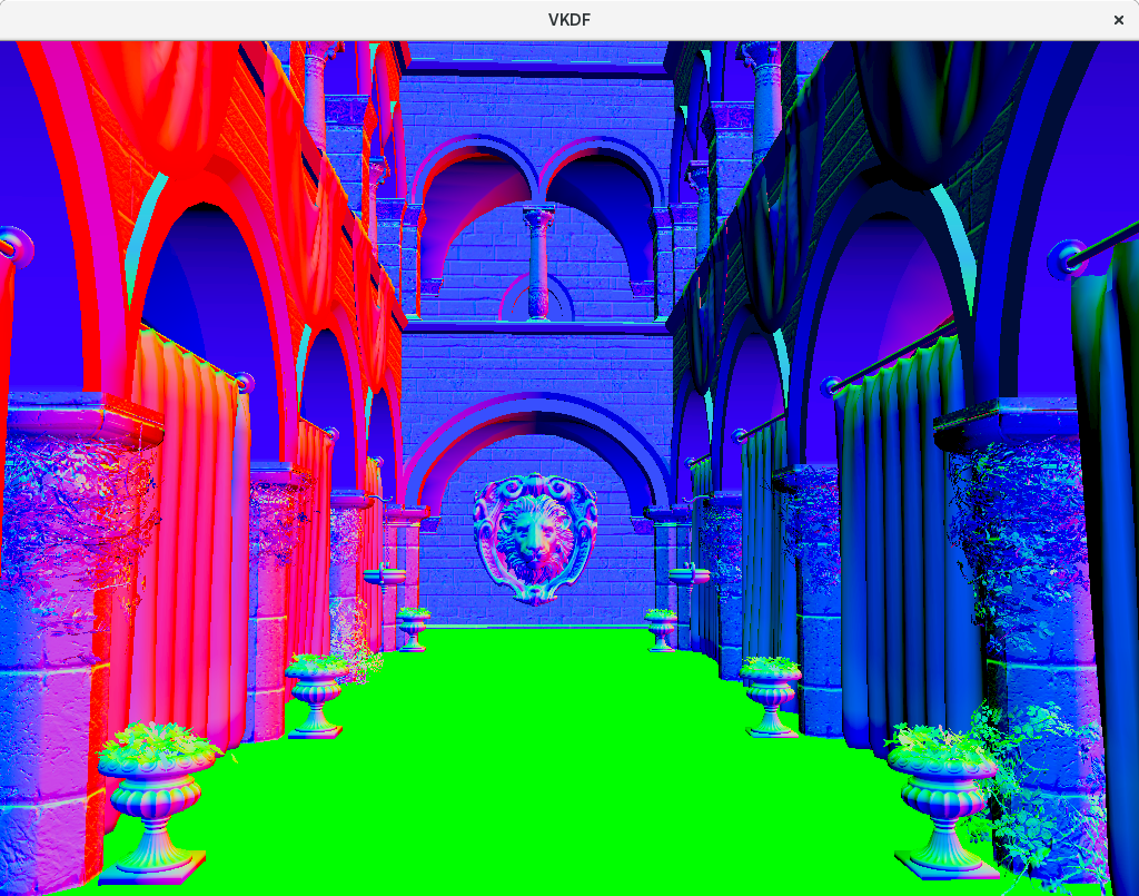
Here we see the normalized normal vectors for each fragment in view-space. This means they are expressed in a coordinate space in which our camera is at the origin and the positive Z direction is opposite to the camera’s view vector. Therefore, we see that surfaces pointing to the right of our camera are red (positive X), those pointing up are green (positive Y) and those pointing opposite to the camera’s view direction are blue (positive Z).
It should be mentioned that some of these surfaces use normal maps for bump mapping. These normal maps are textures that provide per-fragment normal information instead of the usual vertex normals that come with the polygon meshes. This means that instead of computing per-fragment normals as a simple interpolation of the per-vertex normals across the polygon faces, which gives us a rather flat result, we use a texture to adjust the normal for each fragment in the surface, which enables the lighting pass to render more nuanced surfaces that seem to have a lot more volume and detail than they would have otherwise.
For comparison, here is the GBuffer normal texture without bump mapping enabled. The difference in surface detail should be obvious. Just look at the lion figure at the far end or the columns and and you will immediately notice the addditional detail added with bump mapping to the surface descriptions:
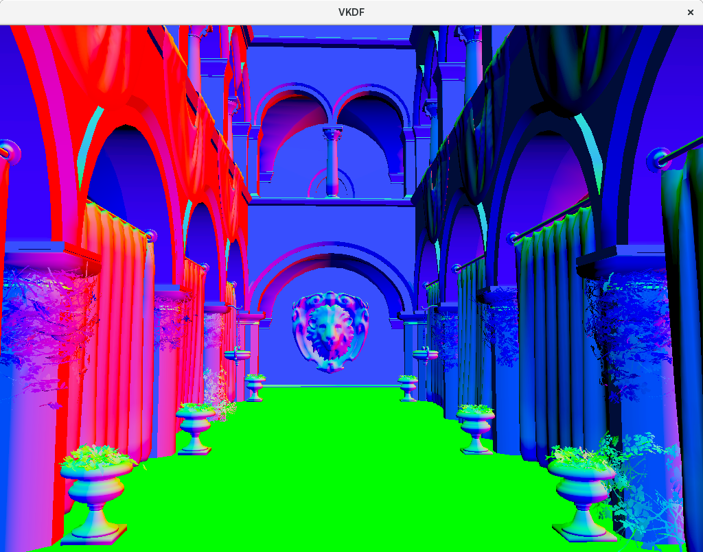
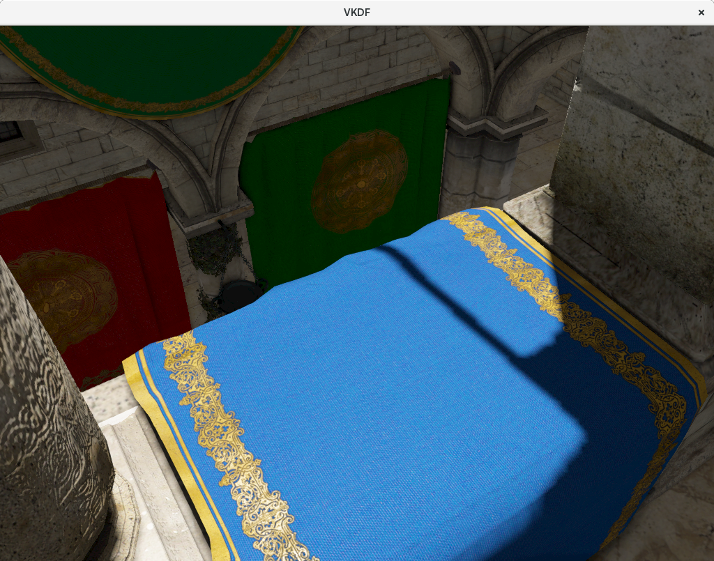
To make the impact of the bump mapping more obvious, here is a different shot of the final rendering focusing on the columns of the upper floor of the atrium, with and without bump mapping:
 |
 |
All the extra detail in the columns is the sole result of the bump mapping technique.
Diffuse color
Here we have the diffuse color of each fragment in the scene. This is basically how our scene would look like if we didn’t implement a lighting pass that considers how the light source interacts with the scene.
Naturally, we will use this information in the lighting pass to modulate the color output based on the light interaction with each fragment.
Specular color

This is similar to the diffuse texture, but here we are storing the color (and strength) used to compute specular reflections.
Similarly to normal textures, we use specular maps to obtain per-fragment specular colors and intensities. This allows us to simulate combinations of more complex materials in the same mesh by specifying different specular properties for each fragment.
For example, if we look at the cloths that hang from the upper floor of the atrium, we see that they are mostly black, meaning that they barely produce any specular reflection, as it is to be expected from textile materials. However, we also see that these same cloths have an embroidery that has specular reflection (showing up as a light gray color), which means these details in the texture have stronger specular reflections than its surrounding textile material:
The image shows visible specular reflections in the yellow embroidery decorations of the cloth (on the bottom-left) that are not present in the textile segment (the blue region of the cloth).
Fragment positions from Light
Finally, we store fragment positions in the coordinate space of the light source so we can implement shadows in the lighting pass. This image may be less intuitive to interpret, since it is encoding space positions from the point of view of the sun rather than physical properties of the fragments. We will need to retrieve this information for each fragment during the lighting pass so that we can tell, together with the shadow map, which fragments are visible from the light source (and therefore are directly lit by the sun) and which are not (and therefore are in the shadows). Again, more detail on how that process works, step by step and including Vulkan source code in my series of posts on that topic.
Step 4: Screen Space Ambient Occlusion
With the information stored in the GBuffer we can now also run a screen-space ambient occlusion pass that we will use to improve our lighting pass later on.
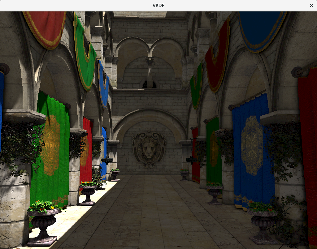
The idea here, as I discussed in my lighting and shadows series, the Phong lighting model simplifies ambient lighting by making it constant across the scene. As a consequence of this, lighting in areas that are not directly lit by a light source look rather flat, as we can see in this image:
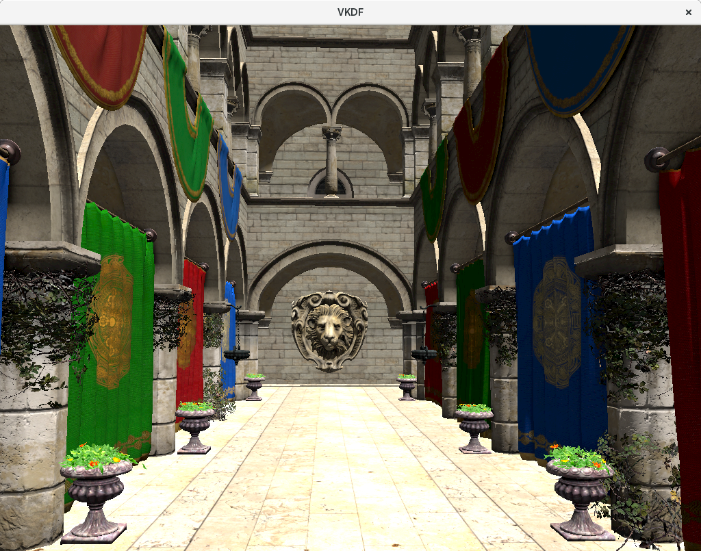
Screen-space Ambient Occlusion is a technique that gathers information about the amount of ambient light occlusion produced by nearby geometry as a way to better estimate the ambient light term of the lighting equations. We can then use that information in our lighting pass to modulate ambient light accordingly, which can greatly improve the sense of depth and volume in the scene, specially in areas that are not directly lit:

Comparing the images above should illustrate the benefits of the SSAO technique. For example, look at the folds in the blue curtains on the right side of the images, without SSAO, we barely see them because the lighting is too flat across all the pixels in the curtain. Similarly, thanks to SSAO we can create shadowed areas from ambient light alone, as we can see behind the cloths that hang from the upper floor of the atrium or behind the vines on the columns.
To produce this result, the output of the SSAO pass is a texture with ambient light intensity information that looks like this (after some blur post-processing to eliminate noise artifacts):
In that image, white tones represent strong light intensity and black tones represent low light intensity produced by occlusion from nearby geometry. In our lighting pass we will source from this texture to obtain per-fragment ambient occlusion information and modulate the ambient term accordingly, bringing the additional volume showcased in the image above to the final rendering.
Step 6: Lighting pass
Finally, we get to the lighting pass. Most of what we showcased above was preparation work for this.
The lighting pass mostly goes as I described in my lighting and shadows series, only that since we are doing deferred rendering we get our per-fragment lighting inputs by reading from the GBuffer textures instead of getting them from the vertex shader.
Basically, the process involves retrieving diffuse, ambient and specular color information from the GBuffer and use it as input for the lighting equations to produce the final color for each fragment. We also sample from the shadow map to decide which pixels are in the shadows, in which case we remove their diffuse and specular components, making them darker and producing shadows in the image as a result.
We also use the SSAO output to improve the ambient light term as described before, multipliying the ambient term of each fragment by the SSAO value we computed for it, reducing the strength of the ambient light for pixels that are surrounded by nearby geometry.
The lighting pass is also where we put bump mapping to use. Bump mapping provides more detailed information about surface normals, which the lighting pass uses to simulate more complex lighting interactions with mesh surfaces, producing significantly enhanced results, as I showcased earlier in this post.
After combining all this information, the lighting pass produces an output like this. Compare it with the GBuffer diffuse texture to see all the stuff that this pass is putting together:
Step 7: Tone mapping
After the lighting pass we run a number of post-processing passes, of which tone mapping is the first one. The idea behind tone mapping is this: normally, shader color outputs are limited to the range [0, 1], which puts a hard cap on our lighting calculations. Specifically, it means that when our light contributions to a particular pixel go beyond 1.0 in any color component, they get clamped, which can distort the resulting color in unrealistic ways, specially when this happens during intermediate lighting calculations (since the deviation from the physically correct color is then used as input to more computations, which then build on that error).
To work around this we do our lighting calculations in High Dynamic Range (HDR) which allows us to produce color values with components larger than 1.0, and then we run a tone mapping pass to re-map the result to the [0, 1] range when we are done with the lighting calculations and we are ready for display.
The nice thing about tone mapping is that it gives the developer control over how that mapping happens, allowing us to decide if we are interested in preserving more detail in the darker or brighter areas of the scene.
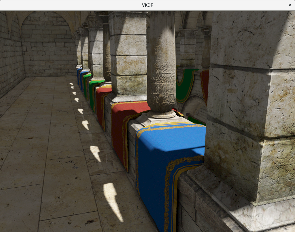
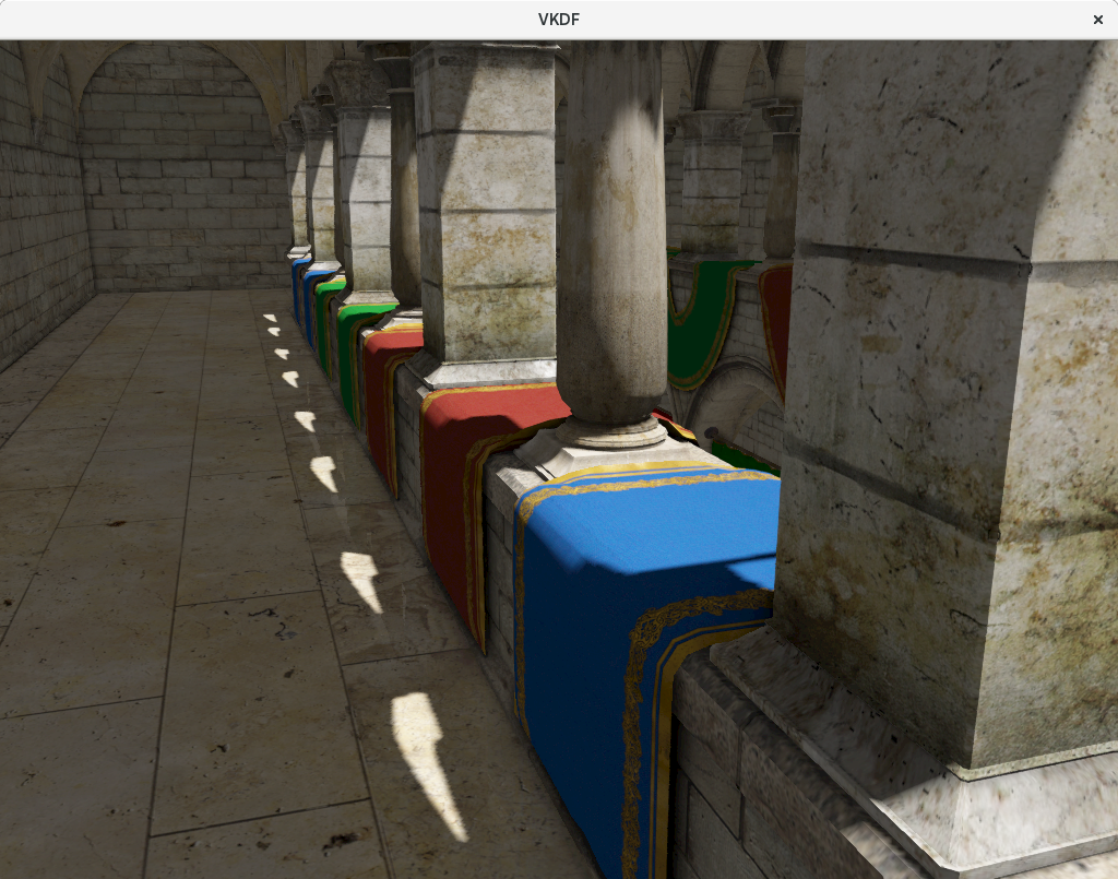
In this particular demo, I used HDR rendering to ramp up the intensity of the sun light beyond what I could have represented otherwise. Without tone mapping this would lead to unrealistic lighting in areas with strong light reflections, since would exceed the 1.0 per-color-component cap and lead to pure white colors as result, losing the color detail from the original textures. This effect can be observed in the following pictures if you look at the lit area of the floor. Notice how the tone-mapped picture better retains the detail of the floor texture while in the non tone-mapped version the floor seems to be over-exposed to light and large parts of it just become white as a result (shadow mapping has been disabled to better showcase the effects of tone-mapping on the floor):
 |
 |
Step 8: Screen Space Reflections (SSR)
The material used to render the floor is reflective, which means that we can see the reflections of the surrounding environment on it.
There are various ways to capture reflections, each with their own set of pros and cons. When I implemented my OpenGL terrain rendering demo I implemented water reflections using “Planar Reflections”, which produce very accurate results at the expense of requiring to re-render the scene with the camera facing in the same direction as the reflection. Although this can be done at a lower resolution, it is still quite expensive and cumbersome to setup (for example, you would need to run an additional culling pass), and you also need to consider that we need to do this for each planar surface you want to apply reflections on, so it doesn’t scale very well. In this demo, although it is not visible in the reference screenshot, I am capturing reflections from the floor sections of both stories of the atrium, so the Planar Reflections approach might have required me to render twice when fragments of both sections are visible (admittedly, not very often, but not impossible with the free camera).
So in this particular case I decided to experiment with a different technique that has become quite popular, despite its many shortcomings, because it is a lot faster: Screen Space Reflections.
As all screen-space techniques, the technique uses information already present in the screen to capture the reflection information, so we don’t have to render again from a different perspective. This leads to a number of limitations that can produce fairly visible artifacts, specially when there is dynamic geometry involved. Nevertheless, in my particular case I don’t have any dynamic geometry, at least not yet, so while the artifacts are there they are not quite as distracting. I won’t go into the details of the artifacts introduced with SSR here, but for those interested, here is a good discussion.
I should mention that my take on this is fairly basic and doesn’t implement relevant features such as the Hierarchical Z Buffer optimization (HZB) discussed here.
The technique has 3 steps: capturing reflections, applying roughness material properties and alpha blending:
Capturing reflections
I only implemented support for SSR in the deferred path, since like in the case of SSAO (and more generally all screen-space algorithms), deferred rendering is the best match since we are already capturing screen-space information in the GBuffer.
The first stage for this requires to have means to identify fragments that need reflection information. In our case, the floor fragments. What I did for this is to capture the reflectiveness of the material of each fragment in the screen during the GBuffer pass. This is a single floating-point component (in the 0-1 range). A value of 0 means that the material is not reflective and the SSR pass will just ignore it. A value of 1 means that the fragment is 100% reflective, so its color value will be solely the reflection color. Values in between allow us to control the strength of the reflection for each fragment with a reflective material in the scene.
One small note on the GBuffer storage: because this is a single floating-point value, we don’t necessarily need an extra attachment in the GBuffer (which would have some performance penalty), instead we can just put this in the alpha component of the diffuse color, since we were not using it (the Intel Mesa driver doesn’t support rendering to RGB textures yet, so since we are limited to RGBA we might as well put it to good use).
Besides capturing which fragments are reflective, we can also store another piece of information relevant to the reflection computations: the material’s roughness. This is another scalar value indicating how much blurring we want to apply to the resulting reflection: smooth metal-like surfaces can have very sharp reflections but with rougher materials that have not smooth surfaces we may want the reflections to look a bit blurry, to better represent these imperfections.
Besides the reflection and roughness information, to capture screen-space reflections we will need access to the output of the previous pass (tone mapping) from which we will retrieve the color information of our reflection points, the normals that we stored in the GBuffer (to compute reflection directions for each fragment in the floor sections) and the depth buffer (from the depth-prepass), so we can check for reflection collisions.
The technique goes like this: for each fragment that is reflective, we compute the direction of the reflection using its normal (from the GBuffer) and the view vector (from the camera and the fragment position). Once we have this direction, we execute a ray marching from the fragment position, in the direction of the reflection. For each point we generate, we take the screen-space X and Y coordinates and use them to retrieve the Z-buffer depth for that pixel in the scene. If the depth buffer value is smaller than our sample’s it means that we have moved past foreground geometry and we stop the process. If we got to this point, then we can do a binary search to pin-point the exact location where the collision with the foreground geometry happens, which will give us the screen-space X and Y coordinates of the reflection point. Once we have that we only need to sample the original scene (the output from the tone mapping pass) at that location to retrieve the reflection color.
As discussed earlier, the technique has numerous caveats, which we need to address in one way or another and maybe adapt to the characteristics of different scenes so we can obtain the best results in each case.
The output of this pass is a color texture where we store the reflection colors for each fragment that has a reflective material:

Naturally, the image above only shows reflection data for the pixels in the floor, since those are the only ones with a reflective material attached. It is immediately obvious that some pixels lack reflection color though, this is due to the various limitations of the screen-space technique that are discussed in the blog post I linked above.
Because the reflections will be alpha-blended with the original image, we use the reflectiveness that we stored in the GBuffer as the base for the alpha component of the reflection color as well (there are other aspects that can contribute to the alpha component too, but I won’t go into that here), so the image above, although not visible in the screenshot, has a valid alpha channel.
Considering material roughness
Once we have captured the reflection image, the next step is to apply the material roughness settings. We can accomplish this with a simple box filter based on the roughness of each fragment: the larger the roughness, the larger the box filter we apply and the blurrier the reflection we get as a result. Because we store roughness for each fragment in the GBuffer, we can have multiple reflective materials with different roughness settings if we want. In this case, we just have one material for the floor though.
Alpha blending
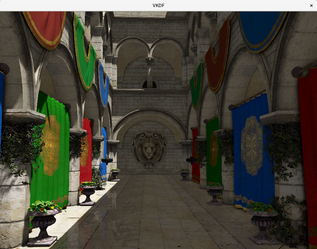
Finally, we use alpha blending to incorporate the reflection onto the original image (the output from the tone mapping) ot incorporate the reflections to the final rendering:
Step 9: Anti-aliasing (FXAA)
So far we have been neglecting anti-aliasing. Because we are doing deferred rendering Multi-Sample Anti-Aliasing (MSAA) is not an option: MSAA happens at rasterization time, which in a deferred renderer occurs before our lighting pass (specifically, when we generate the GBuffer), so it cannot account for the important effects that the lighting pass has on the resulting image, and therefore, on the eventual aliasing that we need to correct. This is why deferred renderers usually do anti-aliasing via post-processing.
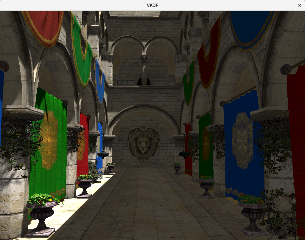
In this demo I have implemented a well-known anti-aliasing post-processing pass known as Fast Approximate Anti Aliasing (FXAA). The technique attempts to identify strong contrast across neighboring pixels in the image to identify edges and then smooth them out using linear filtering. Here is the final result which matches the one I included as reference at the top of this post:
The image above shows the results of the anti-aliasing pass. Compare that with the output of the SSR pass. You can see how this pass has effectively removed the jaggies observed in the cloths hanging from the upper floor for example.
Unlike MSAA, which acts on geometry edges only, FXAA works on all pixels, so it can also smooth out edges produced by shaders or textures. Whether that is something we want to do or not may depend on the scene. Here we can see this happening on the foreground column on the left, where some of the imperfections of the stone are slightly smoothed out by the FXAA pass.
Conclusions and source code
So that’s all, congratulations if you managed to read this far! In the past I have found articles that did frame analysis like this quite interesting so it’s been fun writing one myself and I only hope that this was interesting to someone else.
This demo has been implemented in Vulkan and includes a number of configurable parameters that can be used to tweak performance and quality. The work-in-progress source code is available here, but beware that I have only tested this on Intel, since that is the only hardware I have available, so you may find issues if you run this on other GPUs. If that happens, let me know in the comments and I might be able to provide fixes at some point.