The problem of storing the damage
This article is a continuation of the series on damage propagation. While the previous article laid some foundation on the subject, this one discusses the cost (increased CPU and memory utilization) that the feature incurs, as this is highly dependent on design decisions and the implementation of the data structure used for storing damage information.
From the perspective of this article, the two key things worth remembering from the previous one are:
- The damage propagation is an optional WPE/GTK WebKit feature that — when enabled — reduces the browser’s GPU utilization at the expense of increased CPU and memory utilization.
- On the implementation level, the damage is almost always a collection of rectangles that cover the changed region.
The damage information #
Before diving into the problem and its solutions, it’s essential to understand basic properties of the damage information.
The damage nature #
As mentioned in the section about damage of the previous article, the damage information describes a region that changed and requires repainting. It was also pointed out that such a description is usually done via a collection of rectangles. Although sometimes it’s better to describe a region in a different way, the rectangles are a natural choice due to the very nature of the damage in the web engines that originates from the box model.
A more detailed description of the damage nature can be inferred from the Pipeline details section of the previous article. The bottom line is, in the end, the visual changes to the render tree yield the damage information in the form of rectangles. For the sake of clarity, such original rectangles may be referred to as raw damage.
In practice, the above means that it doesn’t matter whether, e.g. the circle is drawn on a 2D canvas or the background color of some block element changes — ultimately, the rectangles (raw damage) are always produced in the process.
Approximating the damage #
As the raw damage is a collection of rectangles describing a damaged region, the geometrical consequence is that there may be more than one set of rectangles describing the same region. It means that raw damage could be stored by a different set of rectangles and still precisely describe the original damaged region — e.g. when raw damage contains more rectangles than necessary. The example of different approximations of a simple raw damage is depicted in the image below:

Changing the set of rectangles that describes the damaged region may be very tempting — especially when the size of the set could be reduced. However, the following consequences must be taken into account:
- The damaged region could shrink when some damaging information would be lost e.g. if too many rectangles would be removed.
- The damaged region could expand when some damaging information would be added e.g. if too many or too big rectangles would be added.
The first consequence may lead to visual glitches when repainting. The second one, however, causes no visual issues but degrades performance since a larger area (i.e. more pixels) must be repainted — typically increasing GPU usage. This means the damage information can be approximated as long as the trade-off between the extra repainted area and the degree of simplification in the underlying set of rectangles is acceptable.
The approximation mentioned above means the situation where the approximated damaged region covers the original damaged region entirely i.e. not a single pixel of information is lost. In that sense, the approximation can only add extra information. Naturally, the lower the extra area added to the original damaged region, the better.
The approximation quality can be referred to as damage resolution, which is:
- low — when the extra area added to the original damaged region is significant,
- high — when the extra area added to the original damaged region is small.
The examples of low (left) and high (right) damage resolutions are presented in the image below:

The problem #
Given the description of the damage properties presented in the sections above, it’s evident there’s a certain degree of flexibility when it comes to processing damage information. Such a situation is very fortunate in the context of storing the damage, as it gives some freedom in designing a proper data structure. However, before jumping into the actual solutions, it’s necessary to understand the problem end-to-end.
The scale #
The Pipeline details section of the previous article introduced two basic types of damage in the damage propagation pipeline:
- layer damage — the damage tracked separately for each layer,
- frame damage — the damage that aggregates individual layer damages and consists of the final damage of a given frame.
Assuming there are layers and there is some data structure called Damage that can store the damage information, it’s easy to notice that there may be instances
of Damage present at the same time in the pipeline as the browser engine requires:
-
Damageobjects for storing layer damage, -
Damageobject for storing frame damage.
As there may be a lot of layers in more complex web pages, the mentioned above may be a very big number.
The first consequence of the above is that the Damage data structure in general should store the damage information in a very compact way to avoid excessive memory usage when Damage objects
are present at the same time.
The second consequence of the above is that the Damage data structure in general should be very performant as each of Damage objects may be involved into a considerable amount of processing when there are
lots of updates across the web page (and hence huge numbers of damage rectangles).
To better understand the above consequences, it’s essential to examine the input and the output of such a hypothetical Damage data structure more thoroughly.
The input #
There are 2 kinds of Damage data structure input:
- other
Damage, - raw damage.
The Damage becomes an input of other Damage in some situations, happening in the middle of the damage propagation pipeline when the broader damage is being assembled from smaller chunks of damage. What it consists
of depends purely on the Damage implementation.
The raw damage, on the other hand, becomes an input of the Damage always at the very beginning of the damage propagation pipeline. In practice, it consists of a set of rectangles that are potentially overlapping, duplicated, or empty. Moreover,
such a set is always as big as the set of changes causing visual impact. Therefore, in the worst case scenario such as drawing on a 2D canvas, the number of rectangles may be enormous.
Given the above, it’s clear that the hypothetical Damage data structure should support 2 distinct input operations in the most performant way possible:
add(Damage),add(Rectangle).
The output #
When it comes to the Damage data structure output, there are 2 possibilities either:
- other
Damage, - the platform API.
The Damage becomes the output of other Damage on each Damage-to-Damage append that was described in the subsection above.
The platform API, on the other hand, becomes the output of Damage at the very end of the pipeline e.g. when the platform API consumes the frame damage (as described in the
pipeline details section of the previous article).
In this situation, what’s expected on the output technically depends on the particular platform API. However, in practice, all platforms supporting damage propagation require a set of rectangles that describe the damaged region.
Such a set of rectangles is fed into the platforms via APIs by simply iterating the rectangles describing the damaged region and transforming them to whatever data structure the particular API expects.
The natural consequence of the above is that the hypothetical Damage data structure should support the following output operation — also in the most performant way possible:
forEachRectangle(...).
The problem statement #
Given all the above perspectives, the problem of designing the Damage data structure can be summarized as storing the input damage information to be accessed (iterated) later in a way that:
- the performance of operations for adding and iterating rectangles is maximal (performance),
- the memory footprint of the data structure is minimal (memory footprint),
- the stored region covers the original region and has the area as close to it as possible (damage resolution).
With the problem formulated this way, it’s obvious that this is a multi-criteria optimization problem with 3 criteria:
- performance (maximize),
- memory footprint (minimize),
- damage resolution (maximize).
Damage data structure implementations #
Given the problem of storing damage defined as above, it’s possible to propose various ways of solving it by implementing a Damage data structure. Before diving into details, however, it’s important to emphasize
that the weights of criteria may be different depending on the situation. Therefore, before deciding how to design the Damage data structure, one should consider the following questions:
- What is the proportion between the power of GPU and CPU in the devices I’m targeting?
- What are the memory constraints of the devices I’m targeting?
- What are the cache sizes on the devices I’m targeting?
- What is the balance between GPU and CPU usage in the applications I’m going to optimize for?
- Are they more rendering-oriented (e.g. using WebGL, Canvas 2D, animations etc.)?
- Are they more computing-oriented (frequent layouts, a lot of JavaScript processing etc.)?
Although answering the above usually points into the direction of specific implementation, usually the answers are unknown and hence the implementation should be as generic as possible. In practice, it means the implementation should not optimize with a strong focus on just one criterion. However, as there’s no silver bullet solution, it’s worth exploring multiple, quasi-generic solutions that have been researched as part of Igalia’s work on the damage propagation, and which are the following:
Damagestoring all input rects,- Bounding box
Damage, Damageusing WebKit’sRegion,- R-Tree
Damage, - Grid-based
Damage.
All of the above implementations are being evaluated along the 3 criteria the following way:
- Performance
- by specifying the time complexity of
add(Rectangle)operation asadd(Damage)can be transformed into the series ofadd(Rectangle)operations, - by specifying the time complexity of
forEachRectangle(...)operation.
- by specifying the time complexity of
- Memory footprint
- by specifying the space complexity of
Damagedata structure.
- by specifying the space complexity of
- Damage resolution
- by subjectively specifying the damage resolution.
Damage storing all input rects #
The most natural — yet very naive — Damage implementation is one that wraps a simple collection (such as vector) of rectangles and hence stores the raw damage in the original form.
In that case, the evaluation is as simple as evaluating the underlying data structure.
Assuming a vector data structure and amortized time complexity of insertion, the evaluation of such a Damage implementation is:
- Performance
- insertion is ✅
- iteration is ❌
- Memory footprint
- ❌
- Damage resolution
- perfect ✅
Despite being trivial to implement, this approach is heavily skewed towards the damage resolution criterion. Essentially, the damage quality is the best possible, yet the expense is a very poor performance and substantial memory footprint. It’s because a number of input rects can be a very big number, thus making the linear complexities unacceptable.
The other problem with this solution is that it performs no filtering and hence may store a lot of redundant rectangles. While the empty rectangles can be filtered out in , filtering out duplicates and some of the overlaps (one rectangle completely containing the other) would make insertion . Naturally, such a filtering would lead to a smaller memory footprint and faster iteration in practice, however, their complexities would not change.
Bounding box Damage #
The second simplest Damage implementation one can possibly imagine is the implementation that stores just a single rectangle, which is a minimum bounding rectangle (bounding box) of all the damage
rectangles that were added into the data structure. The minimum bounding rectangle — as the name suggests — is a minimal rectangle that can fit all the input rectangles inside. This is well demonstrated in the picture below:

As this implementation stores just a single rectangle, and as the operation of taking the bounding box of two rectangles is , the evaluation is as follows:
- Performance
- insertion is ✅
- iteration is ✅
- Memory footprint
- ✅
- Damage resolution
- usually low ⚠️
Contrary to the Damage storing all input rects, this solution yields a perfect performance and memory footprint at the expense of low damage resolution. However,
in practice, the damage resolution of this solution is not always low. More specifically:
- in the optimistic cases (raw damage clustered), the area of the bounding box is close to the area of the raw damage inside,
- in the average cases, the approximation of the damaged region suffers from covering significant areas that were not damaged,
- in the worst cases (small damage rectangles on the other ends of a viewport diagonal), the approximation is very poor, and it may be as bad as covering the whole viewport.
As this solution requires a minimal overhead while still providing a relatively useful damage approximation, in practice, it is a baseline solution used in:
- Chromium,
- Firefox,
- WPE and GTK WebKit when
UnifyDamagedRegionsruntime preference is enabled, which means it’s used in GTK WebKit by default.
Damage using WebKit’s Region #
When it comes to more sophisticated Damage implementations, the simplest approach in case of WebKit is to wrap data structure already implemented in WebCore called
Region. Its purpose
is just as the name suggests — to store a region. More specifically, it’s meant to store rectangles describing region in an efficient way both for storage and for access to take advantage
of scanline coherence during rasterization. The key characteristic of the data structure is that it stores rectangles without overlaps. This is achieved by storing y-sorted lists of x-sorted, non-overlapping
rectangles. Another important property is that due to the specific internal representation, the number of integers stored per rectangle is usually smaller than 4. Also, there are some other useful properties
that are, however, not very useful in the context of storing the damage. More details on the data structure itself can be found in the J. E. Steinhart’s paper from 1991 titled
SCANLINE COHERENT SHAPE ALGEBRA
published as part of Graphics Gems II book.
The Damage implementation being a wrapper of the Region was actually used by GTK and WPE ports as a first version of more sophisticated Damage alternative for the bounding box Damage. Just as expected,
it provided better damage resolution in some cases, however, it suffered from effectively degrading to a more expensive variant bounding box Damage in the majority of situations.
The above was inevitable as the implementation was falling back to bounding box Damage when the Region’s internal representation was getting too complex. In essence, it was addressing the Region’s biggest problem,
which is that it can effectively store rectangles in the worst case due to the way it splits rectangles for storing purposes. More specifically, as the Region stores ledges
and spans, each insertion of a new rectangle may lead to splitting existing rectangles. Such a situation is depicted in the image below, where 3 rectangles are being split
into 9:

Putting the above fallback mechanism aside, the evaluation of Damage being a simple wrapper on top of Region is the following:
- Performance
- insertion is ✅
- iteration is ❌
- Memory footprint
- ❌
- Damage resolution
- perfect ✅
Adding a fallback, the evaluation is technically the same as bounding box Damage for above the fallback point, yet with extra overhead. At the same time, for smaller , the above evaluation
didn’t really matter much as in such case all the performance, memory footprint, and the damage resolution were very good.
Despite this solution (with a fallback) yielded very good results for some simple scenarios (when was small enough), it was not sustainable in the long run, as it was not addressing the majority of use cases,
where it was actually a bit slower than bounding box Damage while the results were similar.
R-Tree Damage #
In the pursuit of more sophisticated Damage implementations, one can think of wrapping/adapting data structures similar to quadtrees, KD-trees etc. However, in most of such cases, a lot of unnecessary overhead is added
as the data structures partition the space so that, in the end, the input is stored without overlaps. As overlaps are not necessarily a problem for storing damage information, the list of candidate data structures
can be narrowed down to the most performant data structures allowing overlaps. One of the most interesting of such options is the R-Tree.
In short, R-Tree (rectangle tree) is a tree data structure that allows storing multiple entries (rectangles) in a single node. While the leaf nodes of such a tree store the original rectangles inserted into the data structure, each of the intermediate nodes stores the bounding box (minimum bounding rectangle, MBR) of the children nodes. As the tree is balanced, the above means that with every next tree level from the top, the list of rectangles (either bounding boxes or original ones) gets bigger and more detailed. The example of the R-tree is depicted in the Figure 5 from the Object Trajectory Analysis in Video Indexing and Retrieval Applications paper:
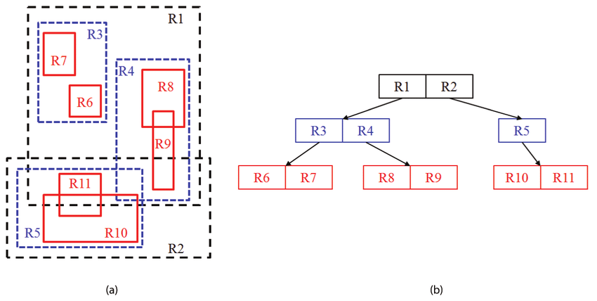
The above perfectly shows the differences between the rectangles on various levels and can also visually suggest some ideas when it comes to adapting such a data structure into Damage:
- The first possibility is to make
Damagea simple wrapper of R-Tree that would just build the tree and allow theDamageconsumer to pick the desired damage resolution on iteration attempt. Such an approach is possible as having the full R-Tree allows the iteration code to limit iteration to a certain level of the tree or to various levels from separate branches. The latter allowsDamageto offer a particularly interesting API where theforEachRectangle(...)function could accept a parameter specifying how many rectangles (at most) are expected to be iterated. - The other possibility is to make
Damagean adaptation of R-Tree that conditionally prunes the tree while constructing it not to let it grow too much, yet to maintain a certain height and hence certain damage quality.
Regardless of the approach, the R-Tree construction also allows one to implement a simple filtering mechanism that eliminates input rectangles being duplicated or contained by existing rectangles on the fly. However, such a filtering is not very effective as it can only consider a limited set of rectangles i.e. the ones encountered during traversal required by insertion.
Damage as a simple R-Tree wrapper
Although this option may be considered very interesting, in practice, storing all the input rectangles in the R-Tree means storing rectangles along with the overhead of a tree structure. In the worst case scenario (node size of 2), the number of nodes in the tree may be as big as , thus adding a lot of overhead required to maintain the tree structure. This fact alone makes this solution have an unacceptable memory footprint. The other problem with this idea is that in practice, the damage resolution selection is usually done once — during browser startup. Therefore, the ability to select damage resolution during runtime brings no benefits while introduces unnecessary overhead.
The evaluation of the above is the following:
- Performance
- insertion is where is the node size ✅
- iteration is where is a parameter and ✅
- Memory footprint
- ❌
- Damage resolution
- low to high ✅
Damage as an R-Tree adaptation with pruning
Considering the problems the previous idea has, the option with pruning seems to be addressing all the problems:
- the memory footprint can be controlled by specifying at which level of the tree the pruning should happen,
- the damage resolution (level of the tree where pruning happens) can be picked on the implementation level (compile time), thus allowing some extra implementation tricks if necessary.
While it’s true the above problems are not existing within this approach, the option with pruning — unfortunately — brings new problems that need to be considered. As a matter of fact, all the new problems it brings are originating from the fact that each pruning operation leads to the loss of information and hence to the tree deterioration over time.
Before actually introducing those new problems, it’s worth understanding more about how insertions work in the R-Tree.
When the rectangle is inserted to the R-Tree, the first step is to find a proper position for the new record (see ChooseLeaf algorithm from Guttman1984). When the target node is found, there are two possibilities:
- adding the new rectangle to the target node does not cause overflow,
- adding the new rectangle to the target node causes overflow.
If no overflow happens, the new rectangle is just added to the target node. However, if overflow happens i.e. the number of rectangles in the node exceeds the limit, the node splitting algorithm is invoked (see SplitNode algorithm from Guttman1984) and the changes are being propagated up the tree (see ChooseLeaf algorithm from Guttman1984).
The node splitting, along with adjusting the tree, are very important steps within insertion as those algorithms are the ones that are responsible for shaping and balancing the tree. For example, when all the nodes in the tree are full and the new rectangle is being added, the node splitting will effectively be executed for some leaf node and all its ancestors, including root. It means that the tree will grow and possibly, its structure will change significantly.
Due to the above mechanics of R-Tree, it can be reasonably asserted that the tree structure becomes better as a function of node splits. With that, the first problem of the tree pruning becomes obvious: tree pruning on insertion limits the amount of node splits (due to smaller node splits cascades) and hence limits the quality of the tree structure. The second problem — also related to node splits — is that with all the information lost due to pruning (as pruning is the same as removing a subtree and inserting its bounding box into the tree) each node split is less effective as the leaf rectangles themselves are getting bigger and bigger due to them becoming bounding boxes of bounding boxes (…) of the original rectangles.
The above problems become more visible in practice when the R-tree input rectangles tend to be sorted. In general, one of the R-Tree problems is that its structure tends to be biased when the input rectangles are sorted. Despite the further insertions usually fix the structure of the biased tree, it’s only done to some degree, as some tree nodes may not get split anymore. When the pruning happens and the input is sorted (or partially sorted) the fixing of the biased tree is much harder and sometimes even impossible. It can be well explained with the example where a lot of rectangles from the same area are inserted into the tree. With the number of such rectangles being big enough, a lot of pruning will happen and hence a lot of rectangles will be lost and replaced by larger bounding boxes. Then, if a series of new insertions will start inserting nodes from a different area which is partially close to the original one, the new rectangles may end up being siblings of those large bounding boxes instead of the original rectangles that could be clustered within nodes in a much more reasonable way.
Given the above problems, the evaluation of the whole idea of Damage being the adaptation of R-Tree with pruning is the following:
- Performance
- insertion is where is the node size, is a parameter, and ✅
- iteration is ✅
- Memory footprint
- ✅
- Damage resolution
- low to medium ⚠️
Despite the above evaluation looks reasonable, in practice, it’s very hard to pick the proper pruning strategy. When the tree is allowed to be taller, the damage resolution is usually better, but the increased memory footprint, logarithmic insertions, and increased iteration time combined pose a significant problem. On the other hand, when the tree is shorter, the damage resolution tends to be low enough not to justify using R-Tree.
Grid-based Damage #
The last, more sophisticated Damage implementation, uses some ideas from R-Tree and forms a very strict, flat structure. In short, the idea is to take some rectangular part of a plane and divide it into cells,
thus forming a grid with columns and rows. Given such a division, each cell of the grid is meant to store at most one rectangle that effectively is a bounding box of the rectangles matched to
that cell. The overview of the approach is presented in the image below:

As the above situation is very straightforward, one may wonder what would happen if the rectangle would span multiple cells i.e. how the matching algorithm would work in that case.
Before diving into the matching, it’s important to note that from the algorithmic perspective, the matching is very important as it accounts for the majority of operations during new rectangle insertion into the Damage data structure.
It’s because when the matched cell is known, the remaining part of insertion is just about taking the bounding box of existing rectangle stored in the cell and the new rectangle, thus having
time complexity.
As for the matching itself, it can be done in various ways:
- it can be done using strategies known from R-Tree, such as matching a new rectangle into the cell where the bounding box enlargement would be the smallest etc.,
- it can be done by maximizing the overlap between the new rectangle and the given cell,
- it can be done by matching the new rectangle’s center (or corner) into the proper cell,
- etc.
The above matching strategies fall into 2 categories:
- matching algorithms that compare a new rectangle against existing cells while looking for the best match,
- matching algorithms that calculate the target cell using a single formula.
Due to the nature of matching, the strategies eventually lead to smaller bounding boxes stored in the Damage and hence to better damage resolution as compared to the
algorithms. However, as the practical experiments show, the difference in damage resolution is not big enough to justify
time complexity over . More specifically, the difference in damage resolution is usually unnoticeable, while the difference between
and insertion complexity is major, as the insertion is the most critical operation of the Damage data structure.
Due to the above, the matching method that has proven to be the most practical is matching the new rectangle’s center into the proper cell. It has time complexity as it requires just a few arithmetic operations to calculate the center of the incoming rectangle and to match it to the proper cell (see the implementation in WebKit). The example of such matching is presented in the image below:

The overall evaluation of the grid-based Damage constructed the way described in the above paragraphs is as follows:
- performance
- insertion is ✅
- iteration is ✅
- memory footprint
- ✅
- damage resolution
- low to high (depending on the ) ✅
Clearly, the fundamentals of the grid-based Damage are strong, but the data structure is heavily dependent on the . The good news is that, in practice, even a fairly small grid such as 8x4
()
yields a damage resolution that is high. It means that this Damage implementation is a great alternative to bounding box Damage as even with very small performance and memory footprint overhead,
it yields much better damage resolution.
Moreover, the grid-based Damage implementation gives an opportunity for very handy optimizations that improve memory footprint, performance (iteration), and damage resolution further.
As the grid dimensions are given a-priori, one can imagine that intrinsically, the data structure needs to allocate a fixed-size array of rectangles with entries to store cell bounding boxes.
One possibility for improvement in such a situation (assuming small ) is to use a vector along with bitset so that only non-empty cells are stored in the vector.
The other possibility (again, assuming small ) is to not use a grid-based approach at all as long as the number of rectangles inserted so far does not exceed . In other words, the data structure can allocate an empty vector of rectangles upon initialization and then just append new rectangles to the vector as long as the insertion does not extend the vector beyond entries. In such a case, when is e.g. 32, up to 32 rectangles can be stored in the original form. If at some point the data structure detects that it would need to store 33 rectangles, it switches internally to a grid-based approach, thus always storing at most 32 rectangles for cells. Also, note that in such a case, the first improvement possibility (with bitset) can still be used.
Summarizing the above, both improvements can be combined and they allow the data structure to have a limited, small memory footprint, good performance, and perfect damage resolution as long as there are not too many damage rectangles. And if the number of input rectangles exceeds the limit, the data structure can still fall-back to a grid-based approach and maintain very good results. In practice, the situations where the input damage rectangles are not exceeding (e.g. 32) are very common, and hence the above improvements are very important.
Overall, the grid-based approach with the above improvements has proven to be the best solution for all the embedded devices tried so far, and therefore, such a Damage implementation is a baseline solution used in
WPE and GTK WebKit when UnifyDamagedRegions runtime preference is not enabled — which means it works by default in WPE WebKit.
Conclusions #
The former sections demonstrated various approaches to implementing the Damage data structure meant to store damage information. The summary of the results is presented in the table below:
| Implementation | Insertion | Iteration | Memory | Overlaps | Resolution |
|---|---|---|---|---|---|
| Bounding box | ✅ | ✅ | ✅ | No | usually low ⚠️ |
| Grid-based | ✅ | ✅ | ✅ | Yes | low to high ✅ (depending on the ) |
| R-Tree (with pruning) | ✅ | ✅ | ✅ | Yes | low to medium ⚠️ |
| R-Tree (without pruning) | ✅ | ✅ | ❌ | Yes | low to high ✅ |
| All rects | ✅ | ❌ | ❌ | Yes | perfect ✅ |
| Region | ✅ | ❌ | ❌ | No | perfect ✅ |
While all the solutions have various pros and cons, the Bounding box and Grid-based Damage implementations are the most lightweight and hence are most useful in generic use cases.
On typical embedded devices — where CPUs are quite powerful compared to GPUs — both above solutions are acceptable, so the final choice can be determined based on the actual use case. If the actual web application
often yields clustered damage information, the Bounding box Damage implementation should be preferred. Otherwise (majority of use cases), the Grid-based Damage implementation will work better.
On the other hand, on desktop-class devices – where CPUs are far less powerful than GPUs – the only acceptable solution is Bounding box Damage as it has a minimal overhead while it sill provides some
decent damage resolution.
The above are the reasons for the default Damage implementations used by desktop-oriented GTK WebKit port (Bounding box Damage) and embedded-device-oriented WPE WebKit (Grid-based Damage).
When it comes to non-generic situations such as unusual hardware, specific applications etc. it’s always recommended to do a proper evaluation to determine which solution is the best fit. Also, the Damage implementations
other than the two mentioned above should not be ruled out, as in some exotic cases, they may give much better results.